Physics · Ch 4 — Motion in a Plane

Position Vector and Displacement

4.7.1

Position Vector and Displacement

To describe motion in a plane, you need two coordinates — unlike motion along a straight line, where one coordinate suffices. The natural tool for this job is the position vector.

The Position Vector

Choose an origin $O$ in the plane. At any instant, the location of a particle is given by the vector drawn from $O$ to the particle. This vector is called the position vector of the particle.

If the particle has coordinates $(x, y)$ with respect to the origin, its position vector $\mathbf{r}$ is written in component form as:

\mathbf{r} = x\,\hat{\mathbf{i}} + y\,\hat{\mathbf{j}}

where $\hat{\mathbf{i}}$ and $\hat{\mathbf{j}}$ are unit vectors along the $x$ - and $y$ -axes respectively. The magnitude of the position vector is the distance of the particle from the origin:

|\mathbf{r}| = \sqrt{x^{2} + y^{2}}

and its direction is given by the angle $\theta$ it makes with the positive $x$ -axis:

\tan\theta = \frac{y}{x}

Note

The position vector is not a fixed quantity — it changes as the particle moves. At every instant, there is a unique position vector.

Displacement

Suppose a particle moves from a point $P$ at time $t$ to a point $P'$ at time $t'$ . Let the position vectors of $P$ and $P'$ be $\mathbf{r}(t)$ and $\mathbf{r}(t')$ respectively.

The displacement vector $\Delta\mathbf{r}$ is defined as the change in the position vector:

\Delta\mathbf{r} = \mathbf{r}(t') - \mathbf{r}(t)

In component form, if $\mathbf{r}(t) = x\,\hat{\mathbf{i}} + y\,\hat{\mathbf{j}}$ and $\mathbf{r}(t') = x'\,\hat{\mathbf{i}} + y'\,\hat{\mathbf{j}}$ , then:

\Delta\mathbf{r} = (x' - x)\,\hat{\mathbf{i}} + (y' - y)\,\hat{\mathbf{j}} = \Delta x\,\hat{\mathbf{i}} + \Delta y\,\hat{\mathbf{j}}

The magnitude of the displacement is:

|\Delta\mathbf{r}| = \sqrt{(\Delta x)^{2} + (\Delta y)^{2}}

Watch out

Displacement is not the same as the distance travelled. Distance is the length of the actual path taken; displacement is the straight-line distance between the initial and final positions, along with its direction. They are equal only when the motion is along a straight line without reversal.

Properties of Vector Addition (Relevant to Displacement)

Since displacement is a vector difference, it obeys the same rules as vector addition. The textbook lists three key properties that apply to all vectors, including position and displacement vectors.

›Proof

Property 1: Commutativity of vector addition

For any two vectors $\mathbf{a}$ and $\mathbf{b}$ :

$\mathbf{a} + \mathbf{b} = \mathbf{b} + \mathbf{a}$

Proof: Construct the parallelogram with sides $\mathbf{a}$ and $\mathbf{b}$ . The diagonal from the common tail to the opposite vertex represents $\mathbf{a} + \mathbf{b}$ . But the same diagonal also represents $\mathbf{b} + \mathbf{a}$ — the order in which you traverse the sides does not change the resultant. Hence the sum is commutative.

›Proof

Property 2: Associativity of vector addition

For any three vectors $\mathbf{a}$ , $\mathbf{b}$ , and $\mathbf{c}$ :

$(\mathbf{a} + \mathbf{b}) + \mathbf{c} = \mathbf{a} + (\mathbf{b} + \mathbf{c})$

Proof: Using the polygon law of addition, first add $\mathbf{a}$ and $\mathbf{b}$ to get $\mathbf{a} + \mathbf{b}$ , then add $\mathbf{c}$ to this resultant. Alternatively, first add $\mathbf{b}$ and $\mathbf{c}$ to get $\mathbf{b} + \mathbf{c}$ , then add $\mathbf{a}$ . In both cases, the final vector from the tail of the first vector to the head of the last vector is the same — the grouping does not affect the sum.

›Proof

Property 3: Additive identity and inverse

There exists a zero vector $\mathbf{0}$ such that for any vector $\mathbf{a}$ :

$\mathbf{a} + \mathbf{0} = \mathbf{a}$

Also, for every vector $\mathbf{a}$ , there exists a vector $-\mathbf{a}$ such that:

$\mathbf{a} + (-\mathbf{a}) = \mathbf{0}$

Proof: The zero vector has zero magnitude and no direction. Adding it to any vector leaves the vector unchanged. The vector $-\mathbf{a}$ has the same magnitude as $\mathbf{a}$ but opposite direction. When added, they cancel each other, giving the zero vector.

Velocity

The average velocity $\overline{\mathbf{v}}$ of a particle over a time interval $\Delta t$ is defined as the displacement divided by the time interval:

\overline{\mathbf{v}} = \frac{\Delta\mathbf{r}}{\Delta t}

The instantaneous velocity $\mathbf{v}$ is the limit of the average velocity as $\Delta t$ approaches zero — that is, the derivative of the position vector with respect to time:

\mathbf{v} = \lim_{\Delta t \to 0} \frac{\Delta\mathbf{r}}{\Delta t} = \frac{d\mathbf{r}}{dt}

In component form, since $\mathbf{r} = x\hat{\mathbf{i}} + y\hat{\mathbf{j}}$ and the unit vectors are constant in time,

\mathbf{v} = \frac{dx}{dt}\,\hat{\mathbf{i}} + \frac{dy}{dt}\,\hat{\mathbf{j}} = v_{x}\,\hat{\mathbf{i}} + v_{y}\,\hat{\mathbf{j}}

The magnitude of the instantaneous velocity is called the speed:

|\mathbf{v}| = \sqrt{v_{x}^{2} + v_{y}^{2}}

The direction of $\mathbf{v}$ at any instant is tangent to the path of the particle at that point.

Acceleration …

Figure 3.12(a) Position vector r. (b) Displacement Δr and average velocity v̄.

Fig. 3.12 — (a) Position vector r. (b) Displacement Δr and average velocity v̄.

Drawn by us to help you understand the concept clearly, and verified to make sure it's accurate. For exams, practice from your textbook's own diagram.

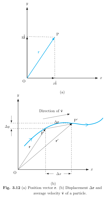
The figure is built around a curved path in the $x$ - $y$ plane. In panel (a), you see a single point $P$ on that path. A straight arrow is drawn from the origin $O$ to $P$ — this is the position vector $\mathbf{r}$ at that instant. Dashed lines drop from the tip of $\mathbf{r}$ down to the $x$ -axis and across to the $y$ -axis, showing that $\mathbf{r}$ has components $x$ and $y$ :

\mathbf{r} = x\,\hat{\mathbf{i}} + y\,\hat{\mathbf{j}}.

Panel (b) zooms out to show two points on the same curved path: $P$ (at time $t$ ) and $P'$ (at a later time $t'$ ). Their position vectors are $\mathbf{r}$ and $\mathbf{r}'$ . A third arrow is drawn from the tip of $\mathbf{r}$ to the tip of $\mathbf{r}'$ — this is the displacement vector $\Delta\mathbf{r}$ :

\Delta\mathbf{r} = \mathbf{r}' - \mathbf{r}.

The arrow for $\Delta\mathbf{r}$ is labelled "Direction of $\bar{\mathbf{v}}$ " because the average velocity $\bar{\mathbf{v}}$ points exactly along $\Delta\mathbf{r}$ :

\bar{\mathbf{v}} = \frac{\Delta\mathbf{r}}{\Delta t}, \quad \Delta t = t' - t.

Dashed projections of $\Delta\mathbf{r}$ onto the $x$ and $y$ axes are also shown, labelled $\Delta x$ and $\Delta y$ . These are the components of the displacement:

\Delta\mathbf{r} = \Delta x\,\hat{\mathbf{i}} + \Delta y\,\hat{\mathbf{j}}.

Important

The displacement $\Delta\mathbf{r}$ is the straight-line chord from $P$ to $P'$ , not the arc length along the curved path. The average velocity $\bar{\mathbf{v}}$ is therefore also a chord-direction quantity. Only when $\Delta t$ becomes infinitesimally small does the chord align with the tangent, giving the instantaneous velocity.

The key formula the textbook develops from this figure is the component form of average velocity:

\bar{\mathbf{v}} = \frac{\Delta x}{\Delta t}\,\hat{\mathbf{i}} + \frac{\Delta y}{\Delta t}\,\hat{\mathbf{j}} = \bar{v}_x\,\hat{\mathbf{i}} + \bar{v}_y\,\hat{\mathbf{j}}.

Each symbol means:

$\mathbf{r}$ — position vector from origin to the particle.
$\mathbf{r}'$ — position vector at a later instant.
$\Delta\mathbf{r}$ — displacement vector (change in position).
$\Delta t$ — time interval between the two instants.
$\bar{\mathbf{v}}$ — average velocity vector.
$\Delta x$ , $\Delta y$ — the $x$ and $y$ components of the displacement.
$\bar{v}_x$ , $\bar{v}_y$ — the $x$ and $y$ components of the average velocity. …

Figure 3.13As Δt→0 the average velocity approaches v, directed along the tangent.

Fig. 3.13 — As Δt→0 the average velocity approaches v, directed along the tangent.

Drawn by us to help you understand the concept clearly, and verified to make sure it's accurate. For exams, practice from your textbook's own diagram.

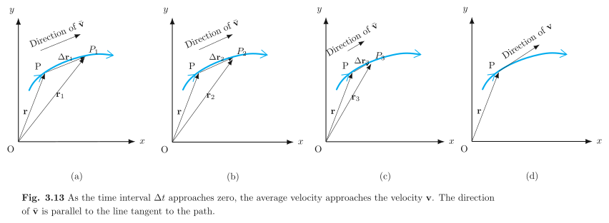
The figure is a sequence of four snapshots that builds the idea of instantaneous velocity from the familiar concept of average velocity. In each panel, you see a curved path — the trajectory of a particle moving in a plane. A fixed point P is marked on this path. In the first panel, a second point P₁ is shown further along the curve, and the straight arrow from P to P₁ represents the displacement vector $\Delta \mathbf{r}_1$ over some time interval $\Delta t_1$ . The average velocity for that interval is $\mathbf{v}_{\text{avg},1} = \Delta \mathbf{r}_1 / \Delta t_1$ , and its direction is exactly along that chord.

The next three panels repeat the same idea but with points P₂, then P₃, each chosen closer and closer to P along the curve. As the second point moves nearer to P, the chord $\Delta \mathbf{r}$ gets shorter, and the direction of the chord rotates to become more and more aligned with the curve itself. By the fourth panel, the second point has merged with P in the limit, and the chord has become a single straight line that just touches the curve — the tangent at P. The arrow drawn along that tangent is labelled "Direction of $\mathbf{v}$ ". That arrow represents the instantaneous velocity $\mathbf{v}$ at the instant the particle passes through P.

The physical idea is straightforward: average velocity over a finite interval points along the chord. As you shrink the interval to zero, the chord's direction approaches the tangent's direction, and the magnitude of the average velocity approaches the instantaneous speed. The textbook uses this geometric limit to define instantaneous velocity in plane motion:

\mathbf{v} = \lim_{\Delta t \to 0} \frac{\Delta \mathbf{r}}{\Delta t} = \frac{d\mathbf{r}}{dt}

Here $\Delta \mathbf{r}$ is the displacement vector (the chord from P to a nearby point), $\Delta t$ is the corresponding time interval, and the limit as $\Delta t \to 0$ gives the derivative $d\mathbf{r}/dt$ . The vector $\mathbf{v}$ is always tangent to the path at the particle's position. Its magnitude $|\mathbf{v}|$ is the instantaneous speed, and its direction is the direction of motion at that instant. …

Figure 3.14Components vx and vy of velocity v and angle θ with x-axis.

Fig. 3.14 — Components vx and vy of velocity v and angle θ with x-axis.

Drawn by us to help you understand the concept clearly, and verified to make sure it's accurate. For exams, practice from your textbook's own diagram.

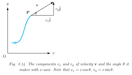
The figure shows a standard $x$ – $y$ coordinate plane with a curved path — the trajectory of a particle moving in two dimensions. At a point labelled $P$ on this path, the instantaneous velocity $\mathbf{v}$ is drawn as an arrow tangent to the curve. From the tip of this arrow, two perpendicular dashed lines drop to the $x$ and $y$ axes, forming a right triangle. The horizontal component is labelled $v_x \hat{\mathbf{i}}$ and the vertical component $v_y \hat{\mathbf{j}}$ , where $\hat{\mathbf{i}}$ and $\hat{\mathbf{j}}$ are the unit vectors along the $x$ and $y$ axes. The angle between $\mathbf{v}$ and the positive $x$ -axis is marked $\theta$ .

The physical idea is that any velocity in the plane can be split into two independent perpendicular parts. The curved path tells you the direction of motion changes, but at the instant shown, the velocity vector's magnitude and direction are fixed. The tangent direction at $P$ is the direction of motion, and the components tell you how fast the particle is moving horizontally and vertically at that instant.

The key formulas the textbook develops from this figure are the resolution of the velocity vector:

v_x = v \cos \theta, \quad v_y = v \sin \theta

Here $v = |\mathbf{v}|$ is the magnitude of the velocity (the speed), $\theta$ is the angle measured from the positive $x$ -axis to the velocity vector, $v_x$ is the $x$ -component (parallel to $\hat{\mathbf{i}}$ ), and $v_y$ is the $y$ -component (parallel to $\hat{\mathbf{j}}$ ). The vector itself is written as $\mathbf{v} = v_x \hat{\mathbf{i}} + v_y \hat{\mathbf{j}}$ .

Watch out

A common mistake is to think $\theta$ is always measured from the horizontal. In this figure it is, but in general problems the reference axis may differ — always check which axis the angle is measured from.

The figure also leads to the inverse relations: given the components, you can find the magnitude and direction: …

Figure 3.15Average acceleration for three intervals Δt1>Δt2>Δt3; (d) limit Δt→0 gives acceleration.

Fig. 3.15 — Average acceleration for three intervals Δt1>Δt2>Δt3; (d) limit Δt→0 gives acceleration.

Drawn by us to help you understand the concept clearly, and verified to make sure it's accurate. For exams, practice from your textbook's own diagram.

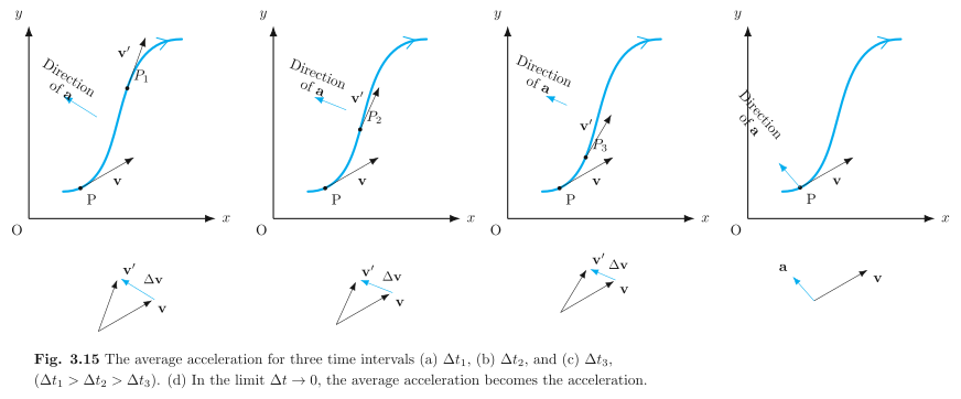
The figure is built around a single curved path in the plane. On that path, three points are marked: P, P₁, P₂, and P₃. The point P is the starting reference. The other three points lie further along the curve, with P₁ closest to P, P₂ farther, and P₃ farthest. The time intervals to reach them from P are labelled Δt₁, Δt₂, and Δt₃, and the caption tells you that Δt₁ > Δt₂ > Δt₃ — so P₁ is reached after the longest time, P₃ after the shortest.

At each of these four points, a velocity vector is drawn tangent to the path. At P the velocity is $\mathbf{v}$ . At P₁, P₂, and P₃ the velocity is the same vector $\mathbf{v}'$ — that is, the figure uses the same final velocity for all three intervals to isolate the effect of the time interval alone. The direction of the average acceleration is indicated along the path, and the key visual point is that as the interval shrinks, the direction of the average acceleration rotates toward the inside of the curve.

The second part of the figure shows a velocity triangle for each interval. You take $\mathbf{v}$ (initial) and $\mathbf{v}'$ (final) and place them tail-to-tail. The vector from the head of $\mathbf{v}$ to the head of $\mathbf{v}'$ is the change in velocity $\Delta \mathbf{v}$ . For the longest interval (Δt₁), $\Delta \mathbf{v}$ is large and points in one direction. For the middle interval (Δt₂), $\Delta \mathbf{v}$ is smaller. For the shortest interval (Δt₃), $\Delta \mathbf{v}$ is smaller still. The triangles are drawn side by side so you can see the vector $\Delta \mathbf{v}$ shrinking and rotating as the time interval decreases.

The third part of the figure (labelled (d)) shows only the point P on the path, with the instantaneous velocity $\mathbf{v}$ drawn tangent to the curve and the instantaneous acceleration $\mathbf{a}$ drawn pointing inward — toward the concave side of the path. This is the limit Δt → 0.

The physical idea. Average acceleration is defined as

\mathbf{a}_{\text{avg}} = \frac{\Delta \mathbf{v}}{\Delta t}.

For a curved path, $\Delta \mathbf{v}$ depends on both the change in speed and the change in direction. As you take smaller and smaller time intervals, the chord between P and the nearby point approaches the tangent, and the direction of $\Delta \mathbf{v}$ approaches a direction perpendicular to the velocity — pointing toward the centre of curvature. In the limit Δt → 0, you get the instantaneous acceleration $\mathbf{a}$ , which is the derivative of the velocity vector with respect to time:

\mathbf{a} = \lim_{\Delta t \to 0} \frac{\Delta \mathbf{v}}{\Delta t} = \frac{d\mathbf{v}}{dt}.

\mathbf{a} = \frac{d\mathbf{v}}{dt}

What each symbol means in context.

$\mathbf{v}$ : velocity at the starting point P.
$\mathbf{v}'$ : velocity at a later point (P₁, P₂, or P₃) — the same vector magnitude and direction is used for all three intervals in the figure.
$\Delta \mathbf{v} = \mathbf{v}' - \mathbf{v}$ : the vector change in velocity over the interval.
$\Delta t$ : the time interval between P and the later point.
$\mathbf{a}_{\text{avg}} = \Delta \mathbf{v} / \Delta t$ : average acceleration over that interval.
$\mathbf{a}$ : instantaneous acceleration at P, the limit of the average acceleration as Δt → 0. …

Start your 14-day free trial to unlock the full solution →

← Previous · 4.7Motion in a Plane Next · 4.7.1 →Example 3.4 — The position of a particle is given by vecr = 3.0thati + 2.0t²hatj + 5…