Economics · Ch 5 — Government Budget and the Economy

Measures of Government Deficit

5.2.1

Measures of Government Deficit

5.2.1 Measures of Government Deficit

When a government spends more than it collects by way of revenue, it incurs a budget deficit. More formally, a budget deficit refers to the excess of total expenditure (both revenue and capital) over total receipts (both revenue and capital). From the 1997–98 budget onwards, the practice of showing budget deficit has been discontinued in India. Instead, economists and policymakers use several specific measures of government deficit, each capturing a different aspect of the government's financial position and carrying its own implications for the economy.

Table 5.1: Receipts and Expenditures of the Central Government, 2023–24 (P.A.)

(figures as per cent of GDP; source: Economic Survey, 2023–24)

#	Item	% of GDP
1	Revenue Receipts (a + b)	9.2
	(a) Tax revenue (net of states' share)	7.9
	(b) Non-tax revenue	1.4
2	Revenue Expenditure, of which	11.8
	(a) Interest payments	3.6
	(b) Major subsidies	1.4
	(c) Defence expenditure	1.0
3	Revenue Deficit (2 − 1)	2.6
4	Capital Receipts (a + b + c), of which	5.8
	(a) Recovery of loans	0.1
	(b) Other receipts (mainly PSU disinvestment)	0.1
	(c) Borrowings and other liabilities	5.6
5	Capital Expenditure	3.2
6	Non-debt Receipts [1 + 4(a) + 4(b)]	9.4
7	Total Expenditure [2 + 5]	1.5 †
	(a) Plan expenditure	–
	(b) Non-plan expenditure	–
8	Fiscal Deficit [7 − 1 − 4(a) − 4(b)]	5.6
9	Primary Deficit [8 − 2(a)]	2.0

Note

† The textbook prints Total Expenditure (item 7) as 1.5% of GDP. By the table's own definition (item 7 = item 2 + item 5), it should be $11.8 + 3.2 = \mathbf{15.0\%}$ of GDP — the printed 1.5 is a misprint. We reproduce the figure exactly as the book prints it and flag the discrepancy rather than silently altering it. The deficit figures below (revenue 2.6%, fiscal 5.6%, primary 2.0%) are the ones the chapter uses.

Revenue Deficit

The revenue deficit is defined as the excess of the government's revenue expenditure over its revenue receipts.

\text{Revenue deficit} = \text{Revenue expenditure} - \text{Revenue receipts}

Revenue deficit includes only those transactions that affect the current income and expenditure of the government. It does not include capital transactions.

When the government incurs a revenue deficit, it implies that the government is dissaving — it is using up the savings of other sectors of the economy to finance a part of its own consumption expenditure. This is a serious situation because it means the government must borrow not only to finance its investment but also to meet its day-to-day consumption requirements. Such borrowing leads to a build-up of the stock of debt and interest liabilities, which forces the government to eventually cut expenditure. Since a major part of revenue expenditure is committed expenditure (salaries, pensions, interest payments, subsidies), it cannot be easily reduced. Often, the government ends up cutting productive capital expenditure or welfare expenditure, which means lower growth and adverse welfare implications.

Watch out

A large revenue deficit is a sign of fiscal indiscipline. It indicates that the government is borrowing to consume, not to invest. This is unsustainable in the long run because it adds to debt without creating assets that generate future income.

Revenue Deficit in the Latest Union Budget

As per the Union Budget 2025–26 (Budget at a Glance, Ministry of Finance, Government of India), the central government's revenue deficit was 1.9 per cent of GDP in 2024–25 (Revised Estimates), and is targeted at 1.5 per cent of GDP for 2025–26 (Budget Estimates).

Fiscal Deficit

The fiscal deficit is the difference between the government's total expenditure and its total receipts excluding borrowing. It is the most comprehensive measure of government deficit and is a key variable in judging the financial health of the public sector and the stability of the economy.

\text{Gross fiscal deficit} = \text{Total expenditure} - (\text{Revenue receipts} + \text{Non-debt creating capital receipts})

Non-debt creating capital receipts are those receipts which are not borrowings and, therefore, do not give rise to debt. Examples include:

Recovery of loans
Proceeds from the sale of Public Sector Undertakings (PSUs) — also called disinvestment receipts

From the financing side, the fiscal deficit can also be expressed as:

\text{Gross fiscal deficit} = \text{Net borrowing at home} + \text{Borrowing from RBI} + \text{Borrowing from abroad}

Net borrowing at home includes borrowing directly from the public through debt instruments (such as small savings schemes) and indirectly from commercial banks through the Statutory Liquidity Ratio (SLR).

Relationship Between Revenue Deficit and Fiscal Deficit

The revenue deficit is a part of the fiscal deficit. The relationship can be seen as:

\text{Fiscal deficit} = \text{Revenue deficit} + \text{Capital expenditure} - \text{Non-debt creating capital receipts}

A large share of revenue deficit in fiscal deficit indicates that a large part of borrowing is being used to meet consumption expenditure needs rather than investment. This is a warning sign for the economy.

Fiscal Deficit in the Latest Union Budget

As per the Union Budget 2025–26 (Budget at a Glance), the fiscal deficit was 4.8 per cent of GDP in 2024–25 (Revised Estimates), and is targeted at 4.4 per cent of GDP for 2025–26 (Budget Estimates) — a continuing path of fiscal consolidation.

Primary Deficit

The borrowing requirement of the government includes interest obligations on accumulated debt. The goal of measuring the primary deficit is to focus on present fiscal imbalances — to obtain an estimate of borrowing on account of current expenditures exceeding revenues, excluding the interest burden of past debt.

\text{Gross primary deficit} = \text{Gross fiscal deficit} - \text{Net interest liabilities}

Net interest liabilities consist of interest payments minus interest receipts by the government on net domestic lending.

The primary deficit tells us how much of the current fiscal deficit is due to current operations (revenue and capital expenditure exceeding non-debt receipts) as opposed to the interest burden inherited from past borrowing. A high primary deficit indicates that the government's current fiscal operations are themselves unsustainable, while a low primary deficit (or a primary surplus) suggests that the government is at least covering its current expenses from current revenues, and the fiscal deficit is largely due to past debt obligations.

Primary Deficit in the Latest Union Budget

As per the same source, the primary deficit was 1.3 per cent of GDP in 2024–25 (Revised Estimates) and is budgeted at 0.8 per cent of GDP for 2025–26. The gap between the fiscal deficit and the primary deficit (about 3.5 per cent of GDP in 2024–25) is accounted for by interest payments on past borrowings.

Deficits of the Central Government — Latest Union Budget Figures

The following table shows the latest official deficit figures (as per cent of GDP):

Deficit measure	2024–25 (Revised Estimates)	2025–26 (Budget Estimates)
Revenue Deficit	1.9	1.5
Fiscal Deficit	4.8	4.4
Primary Deficit	1.3	0.8

Source: Union Budget 2025–26, Budget at a Glance, Ministry of Finance, Government of India.

Note

Your NCERT textbook's own Table 5.1 presents the 2023–24 (P.A.) budget data (revenue deficit 2.6%, fiscal deficit 5.6%, primary deficit 2.0% of GDP). Deficit figures change every year — always mention the year alongside any figure you quote in an exam answer.

How does fiscal policy try to achieve its basic objectives — equity, growth and stability?

Drawn by us to help you understand the concept clearly, and verified to make sure it's accurate. For exams, practice from your textbook's own diagram.

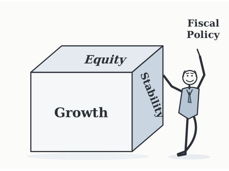
Fiscal policy — the government's use of its budget (taxes, spending and transfers) — is aimed at three broad objectives at once: equity (a fairer distribution of income), growth, and * …

Fiscal Policy and the Determination of Income

Note

Box 5.1 · Fiscal Policy

One of Keynes's central ideas in The General Theory of Employment, Interest and Money was that the government can use fiscal policy — its decisions on spending ( $G$ ), taxes ( $T$ ) and transfers ( $TR$ ) — to stabilise the level of output and employment. By varying these instruments the government seeks to smooth the ups and downs of the economy, in the process running a surplus (when total receipts exceed expenditure) or a deficit budget (when total expenditure exceeds receipts). The analysis that follows introduces the government sector into the earlier income-determination model and shows, step by step, how each fiscal instrument changes the equilibrium level of income through the multiplier.

The Government Sector in the Income Determination Model

The government directly affects the level of equilibrium income in two specific ways:

Government purchases of goods and services ( $G$ ) increase aggregate demand directly.
Taxes and transfers affect the relation between income ( $Y$ ) and disposable income ( $Y_D$ ) — the income available for consumption and saving with households.

Lump-Sum Taxes

Assume the government imposes lump-sum taxes equal to $T$ (taxes that do not depend on income). Also assume the government makes a constant amount of transfers, $\overline{TR}$ .

The consumption function becomes:

C = \overline{C} + cY_D = \overline{C} + c(Y - T + \overline{TR})

where $Y_D = Y - T + \overline{TR}$ is disposable income.

Taxes lower disposable income and consumption. For instance, if one earns ₹1 lakh and has to pay ₹10,000 in taxes, she has the same disposable income as someone who earns ₹90,000 but pays no taxes.

The aggregate demand augmented to include the government is:

AD = \overline{C} + c(Y - T + \overline{TR}) + I + G

Graphically, the lump-sum tax shifts the consumption schedule downward in a parallel way, and hence the aggregate demand curve shifts in a similar fashion.

The income determination condition in the product market is $Y = AD$ , which can be written as:

Y = \overline{C} + c(Y - T + \overline{TR}) + I + G

Solving for the equilibrium level of income:

Y^* = \frac{1}{1-c}(\overline{C} - cT + c\overline{TR} + I + G)

Changes in Government Expenditure

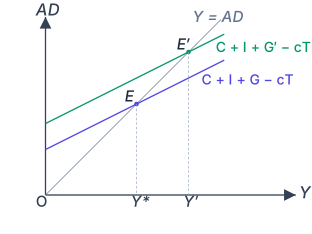
Consider the effects of increasing government purchases ( $G$ ) while keeping taxes constant. When $G$ exceeds $T$ , the government runs a deficit. Since $G$ is a component of aggregate spending, planned aggregate expenditure increases. The aggregate demand schedule shifts up. At the initial level of output, demand exceeds supply and firms expand production.

The government spending multiplier is derived as follows. Suppose $G$ changes to $G + \Delta G$ and as a result $Y$ changes to $Y + \Delta Y$ . Substituting into the equilibrium equation and subtracting the original equation gives:

\Delta Y = \frac{1}{1-c} \Delta G

\frac{\Delta Y}{\Delta G} = \frac{1}{1-c}

Figure 5.1Effect of Higher Government Expenditure

Fig. 5.1 — Effect of Higher Government Expenditure

Drawn by us to help you understand the concept clearly, and verified to make sure it's accurate. For exams, practice from your textbook's own diagram.

Figure 5.1 is a standard Keynesian-cross diagram. The vertical axis is labelled aggregate demand (AD); the horizontal axis is labelled income (Y). A thin 45° line runs from the origin, representing the condition Y = AD — every point on this line is a potential equilibrium where output equals spending.

Two parallel, upward-sloping aggregate demand schedules are drawn. The lower one is labelled C + I + G − cT. It cuts the 45° line at point E, the initial equilibrium. From E, a dashed vertical line drops down to the income axis, marking the initial equilibrium income as Y*.

The second AD schedule is drawn above the first, shifted vertically upward but with the same slope. It is labelled C + I + G' − cT — note the prime on G, indicating a higher level of government spending. This new schedule cuts the 45° line at a higher point, labelled E'. From E', another dashed vertical line drops to the income axis, marking the new equilibrium income as Y'. …

Changes in Taxes

A cut in taxes increases disposable income ( $Y - T$ ) at each level of income. This shifts the aggregate expenditure schedule upward by a fraction $c$ of the decrease in taxes.

The tax multiplier is:

\frac{\Delta Y}{\Delta T} = -\frac{c}{1-c}

Because a tax cut (increase) causes an increase (reduction) in consumption and output, the tax multiplier is a negative multiplier.

Figure 5.2Effect of a Reduction in Taxes

Fig. 5.2 — Effect of a Reduction in Taxes

Drawn by us to help you understand the concept clearly, and verified to make sure it's accurate. For exams, practice from your textbook's own diagram.

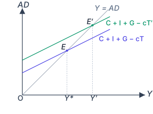
Figure 5.2 is a standard 45°-line (Keynesian cross) diagram. The vertical axis is labelled AD (aggregate demand), and the horizontal axis is labelled Y (national income/output). A 45° line from the origin represents the condition $Y = AD$ — all points where output equals spending.

The initial aggregate demand schedule is a straight line labelled C + I + G − cT. Its intercept on the AD axis is the sum of autonomous components: $C + I + G - cT$ . Its slope is the marginal propensity to consume, $c$ , because induced consumption is $cY$ . This line intersects the 45° line at point E, the initial equilibrium. A dashed vertical line drops from E to the horizontal axis, marking the equilibrium income Y*.

A tax cut is shown: taxes fall from $T$ to $T'$ . This increases disposable income at every level of output, so consumption rises by $c \times (-\Delta T)$ . The aggregate demand schedule shifts parallel upward to a new line labelled C + I + G − cT'. The intercept is now higher by $c\Delta T$ , but the slope remains $c$ — the shift is purely vertical, not a rotation.

The new AD line meets the 45° line at point E', the new equilibrium. Another dashed vertical line from E' marks the new equilibrium income Y' on the horizontal axis. The horizontal distance between Y* and Y' is the change in equilibrium income caused by the tax cut. …

Comparing the two multipliers, the tax multiplier is smaller in absolute value compared to the government spending multiplier. This is because an increase in government spending directly affects total spending, whereas taxes enter the multiplier process through their impact on disposable income, which influences household consumption (which is only a part of total spending). With a $\Delta T$ reduction in taxes, consumption, and hence total spending, increases in the first instance by only $c\Delta T$ .

Why is the poor man crying? Suggest measures to wipe off his tears.

Drawn by us to help you understand the concept clearly, and verified to make sure it's accurate. For exams, practice from your textbook's own diagram.

A heavy, poorly-designed tax burden can weigh most on those least able to bear it. A progressive tax structure and well-targeted transfers/subsidies are the budget's tools for easing that burden — the redi …

Tip

The tax multiplier is always one less in absolute value than the government expenditure multiplier. For example, if the government spending multiplier is 5, the tax multiplier is −4.

The Balanced Budget Multiplier

If an increase in government spending is matched by an equal increase in taxes, so that the budget remains balanced, output will rise by the amount of the increase in government spending.

\text{Balanced budget multiplier} = \frac{\Delta Y}{\Delta G} = \frac{1}{1-c} + \frac{-c}{1-c} = \frac{1-c}{1-c} = 1

A balanced budget multiplier of unity implies that a ₹100 increase in $G$ financed by a ₹100 increase in $T$ increases income by exactly ₹100.

›Proof

To see why the balanced budget multiplier is 1, examine the multiplier process. The increase in government spending by a certain amount raises income by that amount directly and then indirectly through the multiplier chain:

$\Delta Y = \Delta G + c\Delta G + c^2\Delta G + \ldots = \Delta G(1 + c + c^2 + \ldots)$

But the tax increase only enters the multiplier process when the cut in disposable income reduces consumption by $c$ times the reduction in taxes. Thus the effect on income of the tax increase is:

$\Delta Y = -c\Delta T - c^2\Delta T + \ldots = -\Delta T(c + c^2 + \ldots)$

The difference between the two gives the net effect on income. Since $\Delta G = \Delta T$ , we get $\Delta Y = \Delta G$ , that is, income increases by the amount by which government spending increases and the balanced budget multiplier is unity.

This can also be derived from the equilibrium condition. Since investment does not change ( $\Delta I = 0$ ):

$\Delta Y = \Delta G + c(\Delta Y - \Delta T)$

Since $\Delta G = \Delta T$ , we have:

$\frac{\Delta Y}{\Delta G} = \frac{1-c}{1-c} = 1$

Case of Proportional Taxes

A more realistic assumption is that the government collects a constant fraction, $t$ , of income in the form of taxes, so that $T = tY$ .

The consumption function with proportional taxes is:

C = \overline{C} + c(Y - tY + \overline{TR}) = \overline{C} + c(1-t)Y + c\overline{TR}

Proportional taxes not only lower consumption at each level of income but also lower the slope of the consumption function. The marginal propensity to consume out of income falls to $c(1-t)$ .

The new aggregate demand schedule has a larger intercept but is flatter. Now:

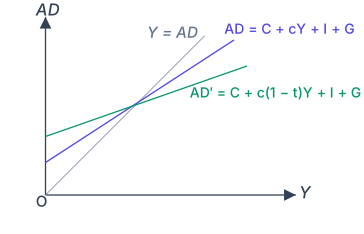
Figure 5.3Government and Aggregate Demand (proportional taxes make the AD schedule flatter)

Fig. 5.3 — Government and Aggregate Demand (proportional taxes make the AD schedule flatter)

Drawn by us to help you understand the concept clearly, and verified to make sure it's accurate. For exams, practice from your textbook's own diagram.

The figure is a standard 45°-line (Keynesian cross) diagram. The vertical axis is labelled AD (Aggregate Demand) and the horizontal axis is Y (Income/Output). A 45° line rising from the origin represents the equilibrium condition $Y = AD$ .

Two aggregate demand schedules are drawn as straight lines crossing the 45° line. The first, labelled AD = C + cY + I + G, corresponds to a lump-sum tax regime. Its slope is $c$ (the marginal propensity to consume out of disposable income), and it has a relatively smaller intercept on the AD axis. The second schedule, labelled AD' = C + c(1 − t)Y + I + G, corresponds to a proportional income tax at rate $t$ . Its intercept is larger than that of the first schedule, but its slope is flatter — $c(1 − t)$ instead of $c$ .

The two lines cross each other at some level of income. No equilibrium points (like $E$ or $E'$ ) are marked on the figure; the diagram is used purely to contrast the slopes and intercepts of the two schedules. …

AD = \overline{C} + c(1-t)Y + c\overline{TR} + I + G = \overline{A} + c(1-t)Y

where $\overline{A} = \overline{C} + c\overline{TR} + I + G$ is autonomous expenditure.

The income determination condition $Y = AD$ gives:

Y = \overline{A} + c(1-t)Y

Solving for the equilibrium level of income:

Y^* = \frac{1}{1-c(1-t)} \overline{A}

The multiplier is:

\frac{\Delta Y}{\Delta \overline{A}} = \frac{1}{1-c(1-t)}

Comparing this with the value of the multiplier with lump-sum taxes, we find that the value has become smaller. When income rose as a result of an increase in government spending in the case of lump-sum taxes, consumption increased by $c$ times the increase in income. With proportional taxes, consumption will rise by less — $c(1-t)$ times the increase in income.

For changes in $G$ , the multiplier is:

\Delta Y = \Delta G + c(1-t)\Delta Y

Figure 5.4Increase in Government Expenditure (with proportional taxes)

Fig. 5.4 — Increase in Government Expenditure (with proportional taxes)

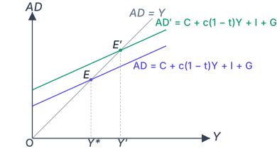
Drawn by us to help you understand the concept clearly, and verified to make sure it's accurate. For exams, practice from your textbook's own diagram.

Figure 5.4 is a Keynesian-cross diagram. It shows two aggregate demand (AD) schedules, both drawn as straight lines with the same slope — flatter than the 45° line. The slope of each AD schedule is $c(1-t)$ , where $c$ is the marginal propensity to consume and $t$ is the proportional tax rate. Because taxes are proportional to income, the slope is smaller than it would be under lump-sum taxes (where the slope would be just $c$ ).

The lower AD schedule is labelled $AD = C + c(1-t)Y + I + G$ . It intersects the 45° line (labelled $AD = Y$ ) at point $E$ . A dashed vertical line drops from $E$ down to the horizontal axis, marking the equilibrium income level $Y^*$ .

The second AD schedule is drawn exactly parallel to the first, but shifted vertically upward. It is labelled $AD' = C + c(1-t)Y + I + G'$ , where $G' > G$ . This new schedule intersects the 45° line at point $E'$ . Another dashed vertical line from $E'$ meets the horizontal axis at $Y'$ , the new equilibrium income.

The key teaching point is the size of the income change. The horizontal distance from $Y^*$ to $Y'$ is noticeably smaller than it would be in the lump-sum tax case (Figure 5.1). The reason is the smaller multiplier. With proportional taxes, the multiplier is $\frac{1}{1 - c(1-t)}$ , which is less than $\frac{1}{1-c}$ . When government spending rises, each round of induced consumption is dampened because a fraction $t$ of any additional income leaks out as taxes. So the same increase in $G$ produces a smaller rise in equilibrium income than it would if taxes were lump-sum. …

Proportional Taxes as an Automatic Stabiliser

The proportional income tax acts as an automatic stabiliser — a shock absorber — because it makes disposable income, and thus consumer spending, less sensitive to fluctuations in GDP.

When GDP rises, disposable income also rises but by less than the rise in GDP because a part of it is siphoned off as taxes. This helps limit the upward fluctuation in consumption spending. During a recession when GDP falls, disposable income falls less sharply, and consumption does not drop as much as it otherwise would have fallen had the tax liability been fixed. This reduces the fall in aggregate demand and stabilises the economy.

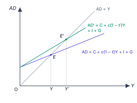
Figure 5.5Effects of a Reduction in the Proportional Tax Rate

Fig. 5.5 — Effects of a Reduction in the Proportional Tax Rate

Drawn by us to help you understand the concept clearly, and verified to make sure it's accurate. For exams, practice from your textbook's own diagram.

Figure 5.5 is an AD–Y diagram. The vertical axis is labelled Aggregate Demand (AD); the horizontal axis is labelled Income/Output (Y). A 45° line from the origin, labelled AD = Y, shows all points where output equals aggregate demand.

Two aggregate demand schedules are drawn, both upward sloping but with different slopes. The original schedule is labelled AD = C + c(1 − t)Y + I + G. It has a positive vertical intercept (autonomous spending) and a slope equal to the marginal propensity to spend out of income, which under proportional taxes is c(1 − t). This schedule intersects the 45° line at point E, and a dashed vertical line from E meets the horizontal axis at Y* — the initial equilibrium income.

The second schedule is labelled AD' = C + c(1 − t')Y + I + G, where t' < t. Because the tax rate is lower, the slope c(1 − t') is larger than c(1 − t). The intercept is unchanged — the tax cut does not affect autonomous spending. So the new schedule pivots upward about the same intercept point, becoming steeper. It intersects the 45° line at a new point E', and a dashed vertical from E' meets the horizontal axis at Y' — the higher equilibrium income.

The key visual point is the rotation, not a parallel shift. A reduction in the proportional tax rate makes the AD line steeper because each rupee of income now leaves more disposable income for consumption. The equilibrium moves from E to E' along the 45° line, and income rises from Y* to Y'. …

Note

Welfare transfers also help to stabilise income. During boom years, when employment is high, tax receipts collected to finance such expenditure increase, exerting a stabilising pressure on high consumption spending. Conversely, during a slump, welfare payments help sustain consumption. Even the private sector has built-in stabilisers — corporations maintain their dividends in the face of a change in income in the short run, and households try to maintain their previous living standards. All these work as shock absorbers without the need for any decision-maker to take action. However, built-in stabilisers reduce only part of the fluctuation in the economy; the rest must be taken care of by deliberate policy initiative.

Discretionary Fiscal Policy

Fiscal policy instruments can be varied to offset the effects of undesirable shifts in investment demand. If investment falls from $I_0$ to $I_1$ , government spending can be raised from $G_0$ to $G_1$ so that autonomous expenditure ( $\overline{C} + I_0 + G_0 = \overline{C} + I_1 + G_1$ ) and equilibrium income remain the same. This deliberate action to stabilise the economy is referred to as discretionary fiscal policy, to distinguish it from the inherent automatic stabilising properties of the fiscal system.

Changes in Transfer Payments

Suppose instead of raising government spending on goods and services, the government increases transfer payments, $\overline{TR}$ . Autonomous spending, $\overline{A}$ , will increase by $c\Delta\overline{TR}$ , so output will rise by less than the amount by which it increases when government expenditure increases, because a part of any increase in transfer payments is saved.

\Delta Y = \frac{c}{1-c} \Delta \overline{TR}

Debt

Budgetary deficits must be financed by either taxation, borrowing, or printing money. Governments have mostly relied on borrowing, giving rise to what is called government debt. The concepts of deficits and debt are closely related. Deficits can be thought of as a flow which add to the stock of debt. If the government continues to borrow year after year, it leads to the accumulation of debt, and the government has to pay more and more by way of interest. These interest payments themselves contribute to the debt.

Perspectives on the Appropriate Amount of Government Debt

There are two interlinked aspects of this issue:

Whether government debt is a burden
The issue of financing the debt

The burden of debt must be discussed keeping in mind that what is true of one small trader's debt may not be true for the government's debt. One must deal with the 'whole' differently from the 'part'. Unlike any one trader, the government can raise resources through taxation and printing money.

By borrowing, the government transfers the burden of reduced consumption to future generations. This is because it borrows by issuing bonds to the people living at present but may decide to pay off the bonds some twenty years later by raising taxes. These may be levied on the young population that have just entered the workforce, whose disposable income will go down and hence consumption. Thus, national savings would fall. Also, government borrowing from the people reduces the savings available to the private sector. To the extent that this reduces capital formation and growth, debt acts as a 'burden' on future generations.

Does the Burden of Debt Really Fall on Future Generations? …

Start your 14-day free trial to unlock the full solution →

← Previous · 5.2Balanced, Surplus and Deficit Budget Next · key-concepts →Key Concepts