Mathematics · Ch 12 — Limits and Derivatives

Intuitive Idea of Derivatives

12.2

Intuitive Idea of Derivatives

The Problem: Finding Instantaneous Velocity

Physical experiments show that a body dropped from a tall cliff covers a distance of $4.9t^2$ metres in $t$ seconds. So the distance $s$ (in metres) as a function of time $t$ (in seconds) is:

s = 4.9t^2

The following table gives the distance travelled, computed from this formula, at a number of instants of time:

$t$ (s)	0	1	1.5	1.8	1.9	1.95	2	2.05	2.1	2.2	2.5	3	4
$s$ (m)	0	4.9	11.025	15.876	17.689	18.63225	19.6	20.59225	21.609	23.716	30.625	44.1	78.4

The goal is to find the velocity of the body at the precise instant $t = 2$ seconds. This is not the same as the average velocity over some interval — it is the instantaneous velocity, the rate of change of distance exactly at $t = 2$ .

We cannot measure velocity at a single instant directly. But we can approach it by examining average velocities over smaller and smaller time intervals that end (or begin) at $t = 2$ , using the distances in the table above. The hope is that these averages will converge to a single number — the instantaneous velocity.

Average Velocity Over Intervals Ending at $t = 2$

Average velocity between $t = t_1$ and $t = t_2$ is:

\text{Average velocity} = \frac{\text{Distance travelled between } t_1 \text{ and } t_2}{t_2 - t_1}

For intervals ending at $t = 2$ , we take $t_2 = 2$ and let $t_1$ be earlier times. The distance travelled from $t_1$ to $2$ is $s(2) - s(t_1) = 19.6 - 4.9t_1^2$ . So:

v_{\text{avg}} = \frac{19.6 - 4.9t_1^2}{2 - t_1}

For instance, taking the whole first two seconds ( $t_1 = 0$ ) gives an average velocity of $19.6/2 = 9.8$ m/s, and taking the interval from $t_1 = 1$ to $t = 2$ gives $(19.6 - 4.9)/1 = 14.7$ m/s. Continuing this for smaller and smaller intervals ending at $t = 2$ gives the following (Table 12.2):

$t_1$	$v$ (m/s)
0	9.8
1	14.7
1.5	17.15
1.8	18.62
1.9	19.11
1.95	19.355
1.99	19.551

As $t_1$ gets closer to 2, the average velocity increases and seems to approach a value just above 19.551 m/s.

Note

This is a left-hand approach — we are looking at intervals that end at $t = 2$ , so we only use data from before $t = 2$ . We are assuming nothing dramatic happens in the last 0.01 seconds before $t = 2$ .

Average Velocity Over Intervals Starting at $t = 2$

Now we reverse the direction: take intervals that begin at $t = 2$ and end at some later time $t_2$ . The average velocity is:

v_{\text{avg}} = \frac{s(t_2) - s(2)}{t_2 - 2} = \frac{4.9t_2^2 - 19.6}{t_2 - 2}

This gives (Table 12.3):

$t_2$	$v$ (m/s)
4	29.4
3	24.5
2.5	22.05
2.2	20.58
2.1	20.09
2.05	19.845
2.01	19.649

As $t_2$ gets closer to 2 from above, the average velocity decreases and approaches a value just below 19.649 m/s.

Watch out

The two sequences approach from opposite sides. The left-hand approach gives values slightly below the limit (increasing to it), while the right-hand approach gives values slightly above the limit (decreasing to it). This is typical — the two sequences should converge to the same number if the function is well-behaved.

Combining the Two Approaches

From the left-hand approach, the average velocity just before $t = 2$ is at least 19.551 m/s. From the right-hand approach, the average velocity just after $t = 2$ is at most 19.649 m/s. Purely on physical grounds, both sequences must approach a common limit. So we can safely conclude:

\text{Instantaneous velocity at } t = 2 \text{ is between } 19.551 \text{ m/s and } 19.649 \text{ m/s}

This is the best estimate we can get from the given discrete data. The true instantaneous velocity — and, equivalently, the derivative of the distance function $s = 4.9t^2$ at $t = 2$ — lies somewhere in that narrow interval. Since velocity is the rate of change of displacement, what we have really done is estimate the rate of change of distance at a single instant, purely from data at nearby instants.

Geometric Interpretation: Slope of the Tangent

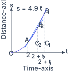
The textbook includes a figure (Fig 12.1) that shows the distance-time curve $s = 4.9t^2$ . On this curve, point A corresponds to $t = 2$ , $s = 19.6$ .

Consider a sequence of points $C_1, C_2, C_3, \dots$ on the time axis, approaching $t = 2$ . The corresponding points on the curve are $B_1, B_2, B_3, \dots$ . The average velocity over the interval $AC_1$ is the slope of the chord $AB_1$ :

$\text{Slope of } AB_1 = \frac{C_1B_1}{AC_1} = \frac{s(2) - s(t_1)}{2 - t_1}$ …

Figure 12.1Distance s = 4.9t² vs time; chords from A approach the tangent as the interval shrinks

Fig. 12.1 — Distance s = 4.9t² vs time; chords from A approach the tangent as the interval shrinks

Drawn by us to help you understand the concept clearly, and verified to make sure it's accurate. For exams, practice from your NCERT textbook's own diagram.

The figure plots the distance $s$ (in metres) against time $t$ (in seconds) for the function $s = 4.9t^{2}$ . The curve is a rising parabola, starting at the origin $O$ . A specific point $A$ is marked on this curve at $t = 2$ seconds; its height is $s = 4.9 \times 2^{2} = 19.6$ metres.

Two other points, $B_{1}$ and $B_{2}$ , lie further up the curve at times $t = 2 + t_{1}$ and $t = 2 + t_{2}$ respectively, where $t_{1}$ and $t_{2}$ are small positive numbers. The figure draws two blue secant chords: one from $A$ to $B_{2}$ , and another from $A$ to $B_{1}$ . Dashed vertical lines are drawn at $t = 2$ , $t = 2 + t_{2}$ , and $t = 2 + t_{1}$ ; a dashed horizontal line is drawn at the height of $A$ (i.e., at $s = 19.6$ ). The axes are labelled Distance (vertical) and Time (horizontal).

The physical idea is this: the average velocity of the falling body over a time interval that ends at $t = 2$ is the slope of the secant chord joining the start and end points on the $s$ - $t$ graph. For the interval from $t = 2$ to $t = 2 + h$ , the average velocity is

v_{\text{avg}} = \frac{s(2+h) - s(2)}{h} = \frac{4.9(2+h)^{2} - 19.6}{h}.

As $h$ gets smaller — that is, as the second point $B$ moves closer to $A$ along the curve — the secant chord approaches a limiting line: the tangent to the curve at $A$ . The slope of that tangent is the instantaneous velocity at $t = 2$ .

The textbook uses this figure to make the following key point concrete: the sequence of ratios $\frac{C_{1}B_{1}}{AC_{1}}, \frac{C_{2}B_{2}}{AC_{2}}, \frac{C_{3}B_{3}}{AC_{3}}, \dots$ (where $C_{1}B_{1}$ is the vertical distance $s_{1} - s_{0}$ travelled in the time interval $h_{1} = AC_{1}$ , and so on) approaches the slope of the tangent at $A$ as the intervals shrink to zero. This slope is the derivative of $s = 4.9t^{2}$ at $t = 2$ .

\text{Instantaneous velocity at } t = 2 \;=\; \lim_{h \to 0} \frac{s(2+h) - s(2)}{h} \;=\; \text{slope of tangent to } s = 4.9t^{2} \text{ at } t = 2.

Table 12.1Distance $s$ (metres) travelled by a falling body at various times $t$ (seconds) for $s = 4.9t^2$

$t$	$s$
0	0
1	4.9
1.5	11.025
1.8	15.876
1.9	17.689
1.95	18.63225
2	19.6
2.05	20.59225
2.1	21.609
2.2	23.716

Table 12.2Average velocity $v$ between $t = t_1$ and $t = 2$ seconds

| $t_1$ | 0 | 1 | 1.5 | 1.8 | 1.9 | 1.95 | 1.99 |

|---|---|---|---|---|---|---|---| …

Table 12.3Average velocity $v$ between $t = 2$ and $t = t_2$ seconds

| $t_2$ | 4 | 3 | 2.5 | 2.2 | 2.1 | 2.05 | 2.01 |

|---|---|---|---|---|---|---|---| …

Start your 14-day free trial to unlock the full solution →

← Previous · 12.1Introduction Next · 12.3 →Limits

Intuitive Idea of Derivatives