Physics · Ch 9 — Mechanical Properties of Fluids

Viscosity

9.5

Viscosity

9.5 Viscosity

When a fluid flows, different layers of the fluid move at different speeds. Think of water flowing through a pipe: the layer right next to the pipe wall is almost stationary, while the layer at the centre moves fastest. This variation in velocity from one layer to the next is the key to understanding viscosity.

Viscosity is the internal friction of a fluid — the resistance that one layer of fluid offers to the relative motion of an adjacent layer. It is the fluid analogue of friction between solid surfaces. Without viscosity, a stirred cup of tea would keep swirling forever; with viscosity, the motion gradually dies out as the internal friction converts kinetic energy into heat.

The Velocity Gradient and Shear Stress

Consider a fluid confined between two parallel plates, each of area $A$ , separated by a distance $d$ . The bottom plate is fixed. The top plate is pulled with a constant force $F$ , so it moves at a steady speed $v_0$ .

The fluid layer immediately in contact with the top plate sticks to it and moves with speed $v_0$ . The layer in contact with the bottom plate sticks to it and stays at rest. In between, the velocity changes linearly from $0$ to $v_0$ across the gap.

The velocity gradient is the rate at which velocity changes with perpendicular distance from the fixed surface:

\frac{dv}{dy}

where $y$ is measured perpendicular to the plates. For the linear profile described, $\frac{dv}{dy} = \frac{v_0}{d}$ .

The force $F$ required to keep the top plate moving is proportional to the area $A$ and to the velocity gradient. This gives us the defining relation for viscosity:

F = \eta A \frac{dv}{dy}

The constant of proportionality $\eta$ is called the coefficient of viscosity (or simply viscosity) of the fluid.

The shear stress $\tau$ (force per unit area) is therefore:

\tau = \frac{F}{A} = \eta \frac{dv}{dy}

This equation is Newton's law of viscous flow. Fluids that obey it are called Newtonian fluids — water, air, and thin oils are examples. Fluids that do not obey it (like toothpaste, paint, or blood) are non-Newtonian.

Watch out

The velocity gradient $\frac{dv}{dy}$ is often called the rate of shear or shear strain rate. Do not confuse it with the velocity itself — it is the change in velocity per unit perpendicular distance.

Units and Dimensions of Viscosity

From $\eta = \frac{F}{A (dv/dy)}$ , we can work out the SI unit:

\eta = \frac{\text{N}}{\text{m}^2 \cdot (\text{m/s})/\text{m}} = \frac{\text{N}}{\text{m}^2} \cdot \frac{\text{s}}{1} = \text{N s m}^{-2} = \text{Pa s}

So the SI unit of viscosity is the pascal-second (Pa s).

The cgs unit is the poise (P), named after the French physician Jean Poiseuille:

1 \text{ P} = 1 \text{ g cm}^{-1} \text{s}^{-1} = 0.1 \text{ Pa s}

In practice, the centipoise (cP) is often used: $1 \text{ cP} = 10^{-3} \text{ Pa s}$ . For reference, the viscosity of water at $20^\circ\text{C}$ is about $1.0 \text{ cP}$ .

The dimensions of viscosity are $[M L^{-1} T^{-1}]$ .

Stokes' Law

When a small sphere moves through a viscous fluid at a low speed (so that the flow is laminar, not turbulent), the viscous drag force $F_d$ opposing its motion is given by Stokes' law:

F_d = 6 \pi \eta r v

where $r$ is the radius of the sphere, $v$ is its velocity relative to the fluid, and $\eta$ is the viscosity of the fluid.

This result is derived from solving the Navier-Stokes equations for creeping flow (very low Reynolds number), but you only need to know and apply the formula.

Note

Stokes' law applies only when the flow around the sphere is laminar — that is, when the Reynolds number $Re = \frac{\rho v d}{\eta}$ is less than about 0.5. For larger Reynolds numbers, the drag becomes more complex and includes a form drag component.

Terminal Velocity

Consider a small sphere falling under gravity through a viscous fluid. Three forces act on it:

Weight downward: $W = mg = \frac{4}{3}\pi r^3 \rho_s g$ , where $\rho_s$ is the density of the sphere.
Buoyant force upward: $F_b = \frac{4}{3}\pi r^3 \rho_f g$ , where $\rho_f$ is the density of the fluid.
Viscous drag upward (from Stokes' law): $F_d = 6\pi \eta r v$ .

Initially, the sphere accelerates. As its speed increases, the drag force grows. Eventually, the net force becomes zero and the sphere falls at a constant speed — the terminal velocity $v_t$ .

At terminal velocity:

\text{Weight} - \text{Buoyancy} - \text{Drag} = 0

\frac{4}{3}\pi r^3 \rho_s g - \frac{4}{3}\pi r^3 \rho_f g - 6\pi \eta r v_t = 0

\frac{4}{3}\pi r^3 (\rho_s - \rho_f) g = 6\pi \eta r v_t

Solving for $v_t$ :

v_t = \frac{2}{9} \frac{r^2 (\rho_s - \rho_f) g}{\eta}

This is a key result. Notice that $v_t$ is proportional to $r^2$ — larger spheres fall much faster. It is also inversely proportional to $\eta$ : more viscous fluids give a lower terminal velocity. …

Figure 9.12(a) A layer of liquid sandwiched between two parallel glass plates, in which the lower plate is fixed and the upper one is moving to the right with velocity v. (b) velocity distribution for viscous flow in a pipe.

Fig. 9.12 — (a) A layer of liquid sandwiched between two parallel glass plates, in which the lower plate is fixed and the upper one is moving to the right with velocity v. (b) velocity distribution for viscous flow in a pipe.

Drawn by us to help you understand the concept clearly, and verified to make sure it's accurate. For exams, practice from your NCERT textbook's own diagram.

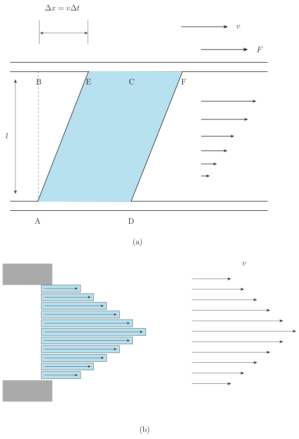
Figure 9.12 in the NCERT textbook is actually two separate diagrams in one, and each teaches a different aspect of viscosity. The two panels are not independent — they work together to show how the same physical idea (internal friction in a fluid) looks in two different geometries: a simple parallel-plate setup and a cylindrical pipe.

Panel (a): the parallel-plate experiment

This is the conceptual starting point. You have two flat glass plates, one fixed at the bottom and the other moving horizontally to the right with a steady velocity $v$ . Between them is a thin layer of liquid of thickness $l$ . The top plate is being pulled by a force $F$ , and in a short time $\Delta t$ it shifts by a distance $\Delta x = v \Delta t$ .

The key visual is the deformation of an imaginary rectangular block of liquid, labelled ABCD. Initially the block is a rectangle. After the top plate moves, the block shears into a parallelogram AEFD — the top edge shifts right while the bottom edge stays put. This shear deformation is the essence of viscosity: the fluid resists this sliding of layers past each other.

From this picture the textbook derives the definition of shear strain rate. The shear strain is $\Delta x / l$ , and the rate at which this strain occurs is $\frac{\Delta x / l}{\Delta t} = \frac{v}{l}$ . The force required to maintain the motion is proportional to the area $A$ of the plates and to this velocity gradient:

F \propto A \frac{v}{l}

The constant of proportionality is the coefficient of viscosity $\eta$ , giving Newton’s law of viscosity for this geometry:

F = \eta \, A \, \frac{v}{l}

F = \eta \, A \, \frac{v}{l}

Watch out

A common mistake is to think $v/l$ is the velocity gradient at a point. It is actually the average velocity gradient across the gap — the velocity changes linearly from 0 at the bottom to $v$ at the top, so the gradient is uniform and equals $v/l$ everywhere.

Panel (b): velocity distribution in a pipe

This panel shows a cross-section of a cylindrical pipe with a parabolic velocity profile. The diagram uses bars or arrows whose lengths represent the speed of the fluid at different radial positions. The longest arrow is at the centre of the pipe, and the arrows get progressively shorter as you move toward the walls, where the velocity is zero.

This is not a separate phenomenon — it is the same viscous behaviour, but now in a cylindrical geometry with a pressure gradient driving the flow. The fluid still obeys Newton’s law of viscosity locally: the shear stress at any radius $r$ is $\tau = -\eta \, \frac{dv}{dr}$ (the negative sign because velocity decreases as $r$ increases). Solving the force balance for a pressure-driven flow in a pipe gives the famous parabolic profile:

v(r) = \frac{P}{4 \eta L} (R^2 - r^2)

where $P$ is the pressure difference across the pipe length $L$ , $R$ is the pipe radius, and $r$ is the radial distance from the centre. …

Figure 9.13Measurement of the coefficient of viscosity of a liquid.

Fig. 9.13 — Measurement of the coefficient of viscosity of a liquid.

Drawn by us to help you understand the concept clearly, and verified to make sure it's accurate. For exams, practice from your NCERT textbook's own diagram.

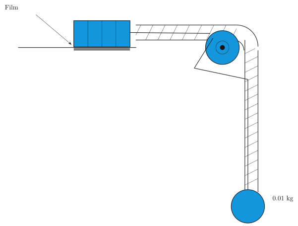
Fig. 9.13 is a schematic of the apparatus used to measure the coefficient of viscosity of a liquid. The figure shows a horizontal table with a thin layer of the test liquid spread over its surface. Resting on this liquid film is a flat block (often called a slider or plate). A string is attached to the block, passes over a pulley at the edge of the table, and has a small mass (0.01 kg) hanging freely at its other end.

The physical idea is straightforward: the hanging mass provides a constant force that tries to pull the block across the table. As the block moves, it drags the liquid film underneath. The liquid resists this motion because of its viscosity — the internal friction between adjacent layers of fluid. The block does not accelerate indefinitely; instead, it quickly reaches a constant (terminal) speed. At that steady speed, the viscous drag force from the liquid exactly balances the weight of the hanging mass (minus any small friction in the pulley, which is usually neglected in the idealised treatment).

The key measurement is this steady speed $v$ of the block. The liquid film has a known thickness $h$ (typically very small, of the order of a millimetre or less), and the block has a known area $A$ in contact with the liquid. The force pulling the block is $F = mg$ , where $m = 0.01\ \text{kg}$ and $g \approx 9.8\ \text{m s}^{-2}$ .

From the definition of viscosity, the viscous force $F$ is proportional to the area $A$ and the velocity gradient across the film. For a thin film with a linear velocity profile (the bottom layer is stationary on the table, the top layer moves with the block's speed $v$ ), the velocity gradient is $v/h$ . So:

F = \eta \, A \, \frac{v}{h}

where $\eta$ is the coefficient of viscosity. Rearranging gives the working formula:

\eta = \frac{F h}{A v} = \frac{m g h}{A v}

Here:

$\eta$ — coefficient of viscosity of the liquid (unit: Pa·s or poise)
$m$ — mass of the hanging weight (0.01 kg)
$g$ — acceleration due to gravity
$h$ — thickness of the liquid film
$A$ — area of the block in contact with the liquid
$v$ — steady speed of the block (measured with a stopwatch and a scale on the table) …

Table 9.2The viscosities of some fluids

Fluid	T (°C)	Viscosity (mPl)
Water	20	1.0
Water	100	0.3
Blood	37	2.7
Machine Oil	16	113
Machine Oil	38	34
Glycerine	20	830
Honey	–	200

Start your 14-day free trial to unlock the full solution →

← Previous · 9.4.2Example 9.7 — A fully loaded Boeing aircraft has a mass of 3.3 × 10⁵kg. Its total wi…Next · 9.5 →Example 9.8 — A metal block of area 0.10m² is connected to a 0.010kg mass via a stri…