Physics · Ch 10 — Thermal Properties of Matter

Conduction

10.9.1

Conduction

The Mechanism of Conduction

Conduction is the transfer of heat through a material without any bulk movement of the material itself. Think of a metal rod held over a flame: the end in your hand gets hot, but the rod itself hasn't moved. What's happening is that energy is being passed from one particle to the next.

In solids, this happens in two ways. In metals, free electrons — which can move easily through the lattice — collide with vibrating atoms and carry kinetic energy rapidly from the hot end to the cold end. In non-metals, the transfer relies entirely on the vibration of atoms in the crystal lattice; hotter atoms vibrate more vigorously and pass that vibration to their neighbours. This is a much slower process than electron-mediated conduction.

Note

Conduction is most efficient in solids, especially metals, because the particles are tightly packed and can transfer energy through direct contact. In gases, the particles are far apart, making conduction extremely slow — that's why air is a good insulator.

Fourier's Law of Heat Conduction

The rate at which heat flows by conduction depends on three things: the temperature difference driving the flow, the material's ability to conduct heat, and the geometry of the object. The French mathematician Joseph Fourier expressed this quantitatively.

Consider a slab of material of cross-sectional area $A$ and thickness $\Delta x$ . One face is at a higher temperature $T_1$ and the other at a lower temperature $T_2$ ( $T_1 > T_2$ ). The amount of heat $Q$ that flows through the slab in a time $t$ is:

Q = \frac{k A (T_1 - T_2) t}{\Delta x}

Here $k$ is the thermal conductivity of the material — a measure of how easily heat flows through it. The larger $k$ is, the faster heat transfers.

The rate of heat flow, or heat current, is $H = Q/t$ . So:

H = \frac{Q}{t} = \frac{k A (T_1 - T_2)}{\Delta x}

This is Fourier's law of heat conduction. It tells us that the heat current is directly proportional to the area and the temperature difference, and inversely proportional to the thickness.

H = \frac{k A (T_1 - T_2)}{\Delta x}

For a thin slab, we can write this in differential form. If the temperature changes by $dT$ over a small distance $dx$ , the heat current is:

H = -k A \frac{dT}{dx}

The negative sign indicates that heat flows from higher temperature to lower temperature — the temperature gradient $\frac{dT}{dx}$ is negative in the direction of heat flow.

Thermal Conductivity of Common Materials

Different materials conduct heat at vastly different rates. Table 10.6 gives the thermal conductivity $k$ for some common substances at standard temperature and pressure, grouped by category.

Table 10.6 Thermal conductivities of some material

Metals

Material	$k$ (J s $^{-1}$ m $^{-1}$ K $^{-1}$ )
Silver	406
Copper	385
Aluminium	205
Brass	109
Steel	50.2
Lead	34.7
Mercury	8.3

Non-metals

Material	$k$ (J s $^{-1}$ m $^{-1}$ K $^{-1}$ )
Insulating brick	0.15
Concrete	0.8
Body fat	0.20
Felt	0.04
Glass	0.8
Ice	1.6
Glass wool	0.04
Wood	0.12
Water	0.8

Gases

Material	$k$ (J s $^{-1}$ m $^{-1}$ K $^{-1}$ )
Air	0.024
Argon	0.016
Hydrogen	0.14

Important

Notice the enormous range: silver conducts heat over 16,000 times better than air. This is why metals feel cold to the touch — they conduct heat away from your hand rapidly — while wood or glass wool feel warm — they trap air and conduct heat very slowly.

Steady State and the Temperature Gradient

When a rod is heated at one end and the other end is kept cool, after some time a steady state is reached. In this state, the temperature at every point along the rod becomes constant in time, though it varies with position. Heat continues to flow, but the temperature profile no longer changes.

In the steady state, the temperature gradient $\frac{dT}{dx}$ is constant along a uniform rod. This means the temperature falls linearly from the hot end to the cold end. If the rod has length $L$ , with the hot end at $T_1$ and the cold end at $T_2$ , then at a distance $x$ from the hot end:

T(x) = T_1 - \frac{(T_1 - T_2)}{L} x

The heat current $H$ is the same through every cross-section of the rod in the steady state.

Watch out

A common mistake is to think that the temperature gradient is the same as the temperature difference. The gradient is the rate of change of temperature with distance — $\frac{dT}{dx}$ — and has units of K/m. The difference $\Delta T$ has units of K. They are related by $\Delta T = \frac{dT}{dx} \cdot L$ only when the gradient is constant.

Conduction Through Composite Slabs

Real walls, windows, and insulation are often made of multiple layers. How do we calculate the heat flow through such a composite?

Consider a slab made of two materials in perfect thermal contact. Material 1 has thickness $L_1$ and thermal conductivity $k_1$ ; material 2 has thickness $L_2$ and thermal conductivity $k_2$ . The outer face of material 1 is at temperature $T_1$ , and the outer face of material 2 is at temperature $T_3$ ( $T_1 > T_3$ ). Let $T_2$ be the temperature at the interface between the two materials.

In the steady state, the same heat current $H$ flows through both materials. Applying Fourier's law to each:

H = \frac{k_1 A (T_1 - T_2)}{L_1} \quad \text{and} \quad H = \frac{k_2 A (T_2 - T_3)}{L_2}

From the first equation: $T_1 - T_2 = \frac{H L_1}{k_1 A}$

From the second: $T_2 - T_3 = \frac{H L_2}{k_2 A}$

Adding these two equations eliminates $T_2$ :

T_1 - T_3 = \frac{H}{A} \left( \frac{L_1}{k_1} + \frac{L_2}{k_2} \right)

Therefore, the heat current through the composite slab is:

H = \frac{A (T_1 - T_3)}{\frac{L_1}{k_1} + \frac{L_2}{k_2}}

Tip

The quantity $\frac{L}{k}$ is called the thermal resistance $R$ of a layer. For a composite slab, the total thermal resistance is the sum of the individual resistances: $R_{\text{total}} = R_1 + R_2 + \dots$ . Then $H = \frac{A \Delta T}{R_{\text{total}}}$ . This is exactly analogous to electrical resistors in series.

The Interface Temperature

We can also find the temperature $T_2$ at the interface between the two materials. From the expression for $H$ through material 1:

T_2 = T_1 - \frac{H L_1}{k_1 A}

Substituting the expression for $H$ :

T_2 = T_1 - \frac{L_1}{k_1 A} \cdot \frac{A (T_1 - T_3)}{\frac{L_1}{k_1} + \frac{L_2}{k_2}}

Simplifying:

T_2 = T_1 - \frac{\frac{L_1}{k_1} (T_1 - T_3)}{\frac{L_1}{k_1} + \frac{L_2}{k_2}}

This can be written more symmetrically as:

T_2 = \frac{\frac{L_1}{k_1} T_3 + \frac{L_2}{k_2} T_1}{\frac{L_1}{k_1} + \frac{L_2}{k_2}}

The interface temperature is a weighted average of the two outer temperatures, with the weights being the thermal resistances of the layers. …

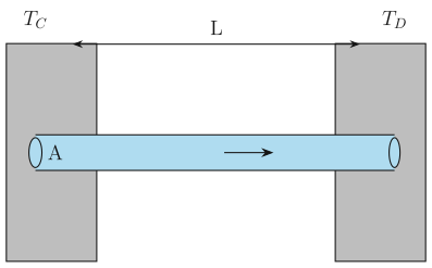
Figure 10.14Steady state heat flow by conduction in a bar with ends at TC and TD (TC > TD).

Fig. 10.14 — Steady state heat flow by conduction in a bar with ends at TC and TD (TC > TD).

Drawn by us to help you understand the concept clearly, and verified to make sure it's accurate. For exams, practice from your NCERT textbook's own diagram.

The figure shows a uniform bar of cross-sectional area $A$ and length $L$ . Its left end is held at a constant temperature $T_C$ and its right end at a lower constant temperature $T_D$ ( $T_C > T_D$ ). A single red arrow runs from the hot end to the cold end, indicating the direction of heat flow. There are no axes, curves, or panels — it is a simple schematic diagram of steady-state conduction.

The physical idea is straightforward: when you maintain a temperature difference across a conductor, heat flows continuously from the hot side to the cold side. After enough time, the temperature at every point in the bar becomes constant in time — this is the steady state. In steady state, the same amount of heat passes through every cross-section per second; the bar does not heat up or cool down anywhere.

The textbook uses this figure to derive the law of thermal conduction. In steady state, the rate of heat transfer $Q/t$ (or power $P$ ) is proportional to:

the cross-sectional area $A$ ,
the temperature difference $(T_C - T_D)$ ,
and inversely proportional to the length $L$ .

The constant of proportionality is the thermal conductivity $k$ , a material property. The result is:

\frac{Q}{t} = k \, A \, \frac{T_C - T_D}{L}

Here $Q$ is the heat transferred in time $t$ , so $Q/t$ is the heat current (in watts). $k$ has units $\text{W m}^{-1} \text{K}^{-1}$ . The fraction $(T_C - T_D)/L$ is the temperature gradient — the slope of the temperature along the bar. In steady state, this gradient is constant for a uniform bar.

Watch out

The formula above assumes the bar is perfectly insulated along its sides — no heat escapes radially. In the figure, the bar is drawn as a simple rectangle with no side arrows, implying this idealisation. In real problems, side losses complicate the gradient.

The figure also sets up the more general form of Fourier's law, which the textbook writes as:

$\frac{Q}{t} = -k \, A \, \frac{dT}{dx}$ …

Start your 14-day free trial to unlock the full solution →

← Previous · 10.9Heat Transfer Next · 10.9.1 →Example 10.6 — What is the temperature of the steel-copper junction in the steady sta…