Economics · Ch 4 — Determination of Income and Employment
The Multiplier Mechanism
The Multiplier Mechanism
The Multiplier Mechanism
The previous section showed that an autonomous expenditure increase of 10 units raised equilibrium income by 50 units (from 250 to 300). This disproportionate change is not a coincidence — it is the result of a chain reaction in the economy. The multiplier mechanism explains exactly how a small initial push gets amplified into a much larger change in total output and income.
How an Initial Expenditure Creates a Chain of Income and Spending
When firms produce final goods, they hire labour, use capital, land, and entrepreneurship. In an economy without indirect taxes or subsidies, the entire value of final output is distributed as factor payments: wages to labour, interest to capital, rent to land, and profit to the entrepreneur. This means that the total value of final output (GDP) equals the total income of the economy (National Income).
Now consider what happens when autonomous expenditure increases by 10. Firms produce 10 units of extra output to meet this new demand. This extra output is sold, and the 10 units of value are distributed as factor payments — so the income of the economy rises by exactly 10.
Here is where the chain begins. People have a marginal propensity to consume (mpc) of 0.8, meaning they spend 80% of any additional income on consumption. So when income rises by 10, consumption expenditure increases by . This creates an excess demand of 8 in the goods market — firms now face demand that is 8 units above the current output.
In the next production cycle, firms increase output by 8 to meet this excess demand. This extra output becomes income for factors of production, raising national income by another 8. With this additional income, consumption rises again by , creating a fresh excess demand of 6.4. Firms respond by increasing output further, and the process repeats.
Round after round, producers expand output to clear each wave of excess demand, while consumers spend a fraction of their new income, generating the next wave. The increments in output become smaller each time because only a fraction (the mpc) of each round's income is spent, but they never quite vanish — they form an infinite geometric series.
The Arithmetic of the Multiplier: Table 4.1
The textbook presents this process in a table that tracks the changes in each round. The key columns are:
- Round 1: The initial autonomous increment of 10 appears as output/income. Consumption demand does not yet respond (it is zero in this round because the income from this output has not yet been received and spent).
- Round 2: Income from round 1 (10) generates consumption of . This becomes the new excess demand, so output increases by .
- Round 3: Income from round 2 () generates consumption of , and output rises by the same amount.
- Round 4: Consumption and output increase by .
- And so on, indefinitely.
| Round | Consumption Demand | Aggregate Demand | Output / Income |
|---|---|---|---|
| 1 | 0 | 10 (autonomous) | 10 |
| 2 | |||
| 3 | |||
| 4 | |||
| ... | ... | ... | ... |
The total increase in output is the sum of all these increments:
This is an infinite geometric series with first term and common ratio . The sum of such a series is , provided . Here:
So the initial autonomous expenditure of 10 leads to a total increase in equilibrium output of 50 — five times the original injection.
Defining the Investment Multiplier
The ratio of the total change in equilibrium output to the initial change in autonomous expenditure is called the investment multiplier (or simply the multiplier). In the example above, the multiplier is .
Let be the total increment in final goods output, (or ) be the initial increment in autonomous expenditure, and be the marginal propensity to consume (mpc). The multiplier is:
Since is the mpc, is the marginal propensity to save (mps). So the multiplier can also be written as .
The size of the multiplier depends entirely on the value of the mpc. A larger mpc (people spend a bigger fraction of additional income) means a larger multiplier. If mpc = 0.9, the multiplier is 10; if mpc = 0.5, the multiplier is 2.
The Paradox of Thrift
Paradox of Thrift
If everyone in the economy decides to save a larger proportion of their income — that is, if the marginal propensity to save rises (or, equivalently, the marginal propensity to consume falls) — the total value of savings in the economy does not increase. It either stays the same or falls. Put differently: as people collectively try to become more thrifty, they end up saving no more than they did before, and sometimes even less. Though it sounds impossible at first, this is a straightforward application of the income-determination model.
Let us see how this works with the same numerical example.
Initially, the economy is in equilibrium at , with and . At this equilibrium, savings are:
Now suppose people suddenly become more thrifty — perhaps due to news of an impending war or economic uncertainty. The mpc drops from 0.8 to 0.5. At the initial income level of 250, this decline in mpc means that consumption spending falls. The reduction in consumption is:
This is an autonomous reduction in consumption expenditure — it happens because people's spending habits have changed, not because income has changed. Aggregate demand therefore falls by 75, creating an excess supply of 75 in the economy. Stocks pile up, and producers cut production by 75 in the next round.
When output falls by 75, income falls by 75. With the new mpc of 0.5, consumption (and hence aggregate demand) falls further by . This creates another excess supply, and producers cut output again by 37.5. The process continues, with each round's reduction being half of the previous round's.
The total reduction in output is the sum of the infinite series:
So the new equilibrium output is:
Now let us calculate savings at this new equilibrium. With and , the equilibrium condition gives , which matches. Savings are:
Savings are still 10 — exactly the same as before! Despite everyone trying to save more, the total savings in the economy have not changed. …
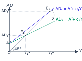
Drawn by us to help you understand the concept clearly, and verified to make sure it's accurate. For exams, practice from your NCERT textbook's own diagram.
Fig. 4.8 illustrates the Paradox of Thrift: when the whole economy tries to save a larger fraction of its income, equilibrium output falls while total saving stays unchanged. The vertical axis is Aggregate Demand () and the horizontal axis is income , with a line from the origin along which .
The crucial point is that both aggregate demand lines are upward-sloping and share the same vertical intercept (here ). They differ only in slope:
- with the larger marginal propensity to consume — the steeper line;
- with the smaller — the flatter line.
A rise in the marginal propensity to save (a fall in mpc from to ) does not shift the line up or down; it reduces the slope, so the line pivots about the common intercept and "swings downwards" — the curved arrow in the figure shows this swing. This is why the caption calls it a downward swing, not a downward shift: the line does not become negatively sloped, it simply becomes flatter.
The steeper line meets the line at , giving the initial equilibrium output ; the flatter line meets it at , giving the lower output . On the vertical axis the equilibrium demand levels are marked and .
Using with :
…