Mathematics · Ch 11 — Three-Dimensional Geometry

Shortest Distance Between Two Lines

11.5

Shortest Distance Between Two Lines

11.5 Shortest Distance Between Two Lines

Concept of Shortest Distance

The shortest distance between two lines in space is the length of the smallest possible segment joining a point on one line to a point on the other.

For intersecting lines, this distance is zero. For parallel lines, it is the perpendicular distance from any point on one line to the other, which is constant.

A third category exists: lines that are neither intersecting nor parallel. These are called skew lines.

Note

Skew lines are non-coplanar — no single plane can contain both lines. This is what distinguishes them from intersecting or parallel lines, which always lie in some common plane.

For example, in a rectangular room of dimensions 1, 3, 2 units along the $x$ , $y$ , and $z$ -axes, the ceiling diagonal $GE$ and the wall diagonal $DB$ are skew — they are not parallel and they never meet.

For skew lines, the segment giving the shortest distance is perpendicular to both lines (the common perpendicular).

Shortest Distance for Skew Lines

The shortest distance between two skew lines is the length of the common perpendicular segment — perpendicular to both lines and joining a point on one to a point on the other.

Vector Form

For two skew lines

\vec{r} = \vec{a}_1 + \lambda \vec{b}_1

\vec{r} = \vec{a}_2 + \mu \vec{b}_2

where $\vec{a}_1$ , $\vec{a}_2$ are position vectors of points on the lines and $\vec{b}_1$ , $\vec{b}_2$ are their direction vectors, the shortest distance is:

d = \frac{|(\vec{b}_1 \times \vec{b}_2) \cdot (\vec{a}_2 - \vec{a}_1)|}{|\vec{b}_1 \times \vec{b}_2|}

Important

The denominator $|\vec{b}_1 \times \vec{b}_2|$ is non-zero because for skew lines the direction vectors are not parallel (otherwise the lines would be parallel, not skew).

Derivation of the Formula

›Proof

The shortest-distance segment is perpendicular to both lines, so its direction is along $\vec{b}_1 \times \vec{b}_2$ . The unit vector along the common perpendicular is

$\hat{n} = \frac{\vec{b}_1 \times \vec{b}_2}{|\vec{b}_1 \times \vec{b}_2|}$

The vector joining a point on $L_1$ (position $\vec{a}_1$ ) to a point on $L_2$ (position $\vec{a}_2$ ) is $\vec{a}_2 - \vec{a}_1$ . The shortest distance $d$ is the magnitude of its projection onto $\hat{n}$ :

$d = |(\vec{a}_2 - \vec{a}_1) \cdot \hat{n}| = \left| (\vec{a}_2 - \vec{a}_1) \cdot \frac{\vec{b}_1 \times \vec{b}_2}{|\vec{b}_1 \times \vec{b}_2|} \right|$

Therefore:

$d = \frac{|(\vec{b}_1 \times \vec{b}_2) \cdot (\vec{a}_2 - \vec{a}_1)|}{|\vec{b}_1 \times \vec{b}_2|}$

Watch out

A common mistake is to forget the absolute value in the numerator. The distance must be positive, so take the absolute value of the scalar triple product.

Cartesian Form

For skew lines in Cartesian form

\frac{x - x_1}{a_1} = \frac{y - y_1}{b_1} = \frac{z - z_1}{c_1}

\frac{x - x_2}{a_2} = \frac{y - y_2}{b_2} = \frac{z - z_2}{c_2}

with points $(x_1, y_1, z_1)$ , $(x_2, y_2, z_2)$ and direction ratios $(a_1, b_1, c_1)$ , $(a_2, b_2, c_2)$ :

d = \frac{\begin{vmatrix} x_2 - x_1 & y_2 - y_1 & z_2 - z_1 \\ a_1 & b_1 & c_1 \\ a_2 & b_2 & c_2 \end{vmatrix}}{\sqrt{(b_1 c_2 - b_2 c_1)^2 + (c_1 a_2 - c_2 a_1)^2 + (a_1 b_2 - a_2 b_1)^2}}

The numerator is the determinant formed by the vector joining the two points and the two direction vectors; the denominator is $|\vec{b}_1 \times \vec{b}_2|$ expressed in Cartesian components.

Shortest Distance Between Parallel Lines

For parallel lines the shortest distance is constant — the perpendicular distance from any point on one line to the other.

Vector Form

For parallel lines

\vec{r} = \vec{a}_1 + \lambda \vec{b}

\vec{r} = \vec{a}_2 + \mu \vec{b}

sharing direction vector $\vec{b}$ :

d = \frac{|(\vec{a}_2 - \vec{a}_1) \times \vec{b}|}{|\vec{b}|}

›Proof

Take $\vec{a}_2 - \vec{a}_1$ joining a point on each line. Then $|(\vec{a}_2 - \vec{a}_1) \times \vec{b}| = |\vec{a}_2 - \vec{a}_1|\,|\vec{b}|\,\sin\theta$ , where $\theta$ is the angle between $\vec{a}_2 - \vec{a}_1$ and $\vec{b}$ . Since $|\vec{a}_2 - \vec{a}_1|\,\sin\theta$ is the perpendicular distance from the point to the other line, dividing by $|\vec{b}|$ gives $d$ .

Cartesian Form

For parallel lines in Cartesian form …

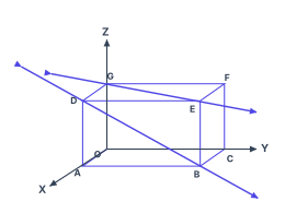
Figure 11.5A room-shaped cuboid on the X, Y, Z axes with vertices O, A, B, C, D, E, F, G showing the two skew lines formed by the ceiling diagonal GE and the wall diagonal DB, each extended with arrows.

Fig. 11.5 — A room-shaped cuboid on the X, Y, Z axes with vertices O, A, B, C, D, E, F, G showing the two skew lines formed by the ceiling diagonal GE and the wall diagonal DB, each extended with arrows.

Drawn by us to help you understand the concept clearly, and verified to make sure it's accurate. For exams, practice from your NCERT textbook's own diagram.

The figure shows a rectangular room drawn as a cuboid with dimensions 1 unit along the $x$ -axis, 3 units along the $y$ -axis, and 2 units along the $z$ -axis. The axes are drawn in an oblique projection so you can see depth. The floor vertices are labelled $O$ (origin), $A$ (on the $x$ -axis), $B$ (the far floor corner), and $C$ (on the $y$ -axis). The ceiling vertices directly above these are $G$ (on the $z$ -axis, above $O$ ), $D$ (above $A$ ), $E$ (above $B$ ), and $F$ (above $C$ ). Two skew lines are drawn in indigo, extended beyond the box with arrows at both ends to show they are infinite lines. One line is $GE$ , the diagonal across the ceiling from $G$ to $E$ . The other line is $DB$ , which runs from $D$ (the ceiling corner directly above $A$ ) diagonally down the wall to $B$ (the floor corner opposite $O$ ).

The physical idea is simple: these two lines are neither parallel nor intersecting. They lie in different planes — $GE$ is entirely in the ceiling plane, $DB$ runs from the ceiling down a wall to the floor — so they are non-coplanar. Such lines are called skew lines. The figure makes it visually clear that no matter how far you extend them, they will never meet, and they are not parallel either. The shortest distance between them is the length of the unique line segment that is perpendicular to both lines.

The textbook uses this figure to introduce the concept of the shortest distance between skew lines. The key formulas developed are:

d = \frac{|(\vec{b}_1 \times \vec{b}_2) \cdot (\vec{a}_2 - \vec{a}_1)|}{|\vec{b}_1 \times \vec{b}_2|}

where:

$\vec{a}_1$ and $\vec{a}_2$ are position vectors of any point on line 1 and line 2 respectively.
$\vec{b}_1$ and $\vec{b}_2$ are direction vectors of line 1 and line 2 respectively.
$\vec{b}_1 \times \vec{b}_2$ is the cross product, giving a vector perpendicular to both lines.
The numerator is the absolute value of the scalar triple product, which gives the volume of the parallelepiped formed by the three vectors. Dividing by the area of the base (the magnitude of the cross product) gives the perpendicular height — that height is the shortest distance. …

Start your 14-day free trial to unlock the full solution →

← Previous · 11.4Example 8 — Find the angle between the pair of lines (x+3)/(3) = (y-1)/(5) = (z+3)…Next · 11.5.1 →Distance Between Two Skew Lines