Physics · Ch 1 — Electric Charges and Fields

Field Due to an Infinitely Long Straight Uniformly Charged Wire

1.14.1

Field Due to an Infinitely Long Straight Uniformly Charged Wire

Why the Field is Radial and Depends Only on $r$

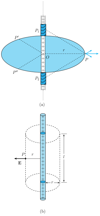
The wire is infinitely long and has a uniform linear charge density $\lambda$ (charge per unit length). This infinite length creates a perfect symmetry: the wire is an axis of symmetry. If you take any point P at a perpendicular distance $r$ from the wire and rotate it around the wire, all such points are equivalent. Therefore:

The magnitude of the electric field $\mathbf{E}$ must be the same at all points that lie at the same radial distance $r$ .
The direction of $\mathbf{E}$ must be radial — pointing directly away from the wire (if $\lambda > 0$ ) or directly toward the wire (if $\lambda < 0$ ). This is because for any pair of symmetric small segments of the wire, the components of their fields perpendicular to the radial direction cancel out, leaving only the radial component.
Since the wire is infinite, the field does not depend on how far along the wire you are — only on the perpendicular distance $r$ .

Thus, the electric field is everywhere radial in a plane perpendicular to the wire, and its magnitude $E$ is a function of $r$ alone.

Using Gauss’s Law to Find $E$

To calculate $E$ , we choose a cylindrical Gaussian surface of radius $r$ and length $l$ , coaxial with the wire.

Flux through the flat ends: The field is radial, so it is parallel to the flat ends (tangential). Hence, the electric flux through both ends is zero.
Flux through the curved surface: At every point on the curved surface, $\mathbf{E}$ is perpendicular (normal) to the surface and has constant magnitude $E$ (since $r$ is constant). The area of the curved surface is $2\pi r l$ .

Therefore, the total electric flux $\Phi$ through the Gaussian surface is:

\Phi = E \times (2\pi r l)

Charge enclosed: The Gaussian surface encloses a length $l$ of the wire. The charge inside is:

q_{\text{enc}} = \lambda l

Now apply Gauss’s law:

\Phi = \frac{q_{\text{enc}}}{\varepsilon_0}

Substitute the expressions:

E \times 2\pi r l = \frac{\lambda l}{\varepsilon_0}

Cancel $l$ (the length of the cylinder) from both sides:

E \times 2\pi r = \frac{\lambda}{\varepsilon_0}

Solve for $E$ :

\boxed{E = \frac{\lambda}{2\pi \varepsilon_0 r}}

Vector Form of the Result

The electric field $\mathbf{E}$ at any point is radial. In vector notation:

\boxed{\mathbf{E} = \frac{\lambda}{2\pi \varepsilon_0 r} \, \hat{\mathbf{n}}}

where:

$\hat{\mathbf{n}}$ is the radial unit vector in the plane perpendicular to the wire, pointing from the wire to the point.
$\lambda$ is the linear charge density (can be positive or negative).
$\varepsilon_0$ is the permittivity of free space.
$r$ is the perpendicular distance from the wire.

Direction:

If $\lambda > 0$ , $\mathbf{E}$ is outward (away from the wire).
If $\lambda < 0$ , $\mathbf{E}$ is inward (toward the wire).

Important Notes …

Figure 1.26(a) Electric field due to an infinitely long thin straight wire is radial, (b) The Gaussian surface for a long thin wire of uniform linear charge density.

Fig. 1.26 — (a) Electric field due to an infinitely long thin straight wire is radial, (b) The Gaussian surface for a long thin wire of uniform linear charge density.

Drawn by us to help you understand the concept clearly, and verified to make sure it's accurate. For exams, practice from your NCERT textbook's own diagram.

The figure is split into two panels, (a) and (b), which together build the physical reasoning and the mathematical result for the electric field of an infinitely long, uniformly charged wire.

Panel (a) establishes the direction of the field. A vertical line of positive charges (the wire) passes through the centre O of a horizontal elliptical plane. Two symmetric elements of the wire, P₁ (above O) and P₂ (below O), are considered. Dashed construction lines connect P₁ to a point P″ on the left rim of the ellipse, P₂ to P′ on the left rim, and both P₁ and P₂ to a point P on the right side of the ellipse at a distance $r$ from O. At P, a fan of three arrows shows the individual electric field contributions from P₁ and P₂, and their vector sum — a single horizontal arrow pointing radially outward from the wire. The key idea is that the components of the fields from P₁ and P₂ perpendicular to the radial direction cancel, leaving only the radial component. Because the wire is infinite, every such symmetric pair of elements produces the same result, so the total electric field $\mathbf{E}$ at any point P is purely radial (outward if the linear charge density $\lambda > 0$ , inward if $\lambda < 0$ ). The points P′ and P″ on the left rim are equivalent to P, confirming that the field magnitude depends only on the radial distance $r$ , not on the position along the wire.

Panel (b) shows the Gaussian surface used to calculate the field magnitude. The wire (a rod of positive charges) is enclosed by a dashed coaxial cylinder of radius $r$ and length $l$ . The cylinder has three parts: a curved side and two flat circular ends. On the left side of the cylinder, an arrow labelled $\mathbf{E}$ points radially outward from the wire, and the distance from the wire to the cylinder surface is marked as $r$ . The length $l$ is dimensioned on the right side of the cylinder. The physical idea is that because the field is radial, the electric flux through the two flat ends is zero (the field is parallel to those surfaces). On the curved part, the field is everywhere perpendicular to the surface and has constant magnitude $E$ (since $r$ is constant). The area of the curved surface is $2\pi r l$ .

Applying Gauss's law, the total electric flux through the Gaussian surface equals the charge enclosed divided by $\varepsilon_0$ :

\Phi = E \cdot (2\pi r l) = \frac{\lambda l}{\varepsilon_0}

Cancelling $l$ (which is non-zero) gives the magnitude of the electric field:

E = \frac{\lambda}{2\pi \varepsilon_0 r}

The vector form is:

$\mathbf{E} = \frac{\lambda}{2\pi \varepsilon_0 r} \hat{\mathbf{n}}$ …

Start your 14-day free trial to unlock the full solution →

← Previous · 1.14Applications of Gauss's Law Next · 1.14.2 →Field Due to a Uniformly Charged Infinite Plane Sheet

Field Due to an Infinitely Long Straight Uniformly Charged Wire