Chemistry · Ch 4 — Chemical Bonding and Molecular Structure

Formation of Molecular Orbitals Linear Combination of Atomic Orbitals (LCAO)

4.7.1

Formation of Molecular Orbitals Linear Combination of Atomic Orbitals (LCAO)

The Need for an Approximate Method

The Schrödinger wave equation gives us wave functions ( $\psi$ ) that describe atomic orbitals. These wave functions represent the amplitude of the electron wave. For a hydrogen atom, the equation can be solved exactly. But for any system with more than one electron — including even the simplest molecule, $H_2$ — an exact solution is impossible. Molecular orbitals, which are one-electron wave functions for the entire molecule, cannot be obtained directly.

To work around this, chemists use an approximate method called the linear combination of atomic orbitals (LCAO). This approach builds molecular orbitals by combining the atomic orbitals of the individual atoms.

Applying LCAO to the Hydrogen Molecule

Consider two hydrogen atoms, labelled A and B. In its ground state, each hydrogen atom has one electron in a 1s orbital. Let the wave function for atom A's 1s orbital be $\psi_A$ , and for atom B's 1s orbital be $\psi_B$ .

The LCAO method states that a molecular orbital ( $\psi_{MO}$ ) can be formed by taking a linear combination of these atomic orbitals. The simplest combinations are addition and subtraction:

\psi_{MO} = \psi_A + \psi_B \quad \text{and} \quad \psi_{MO} = \psi_A - \psi_B

From these two combinations, two distinct molecular orbitals arise:

\sigma = \psi_A + \psi_B

\sigma^* = \psi_A - \psi_B

Figure 4.19Formation of bonding (σ) and antibonding (σ*) molecular orbitals by LCAO of ψA and ψB.

Fig. 4.19 — Formation of bonding (σ) and antibonding (σ*) molecular orbitals by LCAO of ψA and ψB.

Drawn by us to help you understand the concept clearly, and verified to make sure it's accurate. For exams, practice from your NCERT textbook's own diagram.

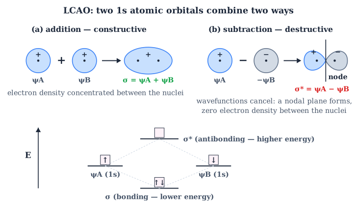
Fig. 4.19 is a schematic that shows what happens when two atomic orbitals — one on atom A and one on atom B — are combined mathematically to form molecular orbitals. The figure does not plot a curve or a graph; instead it uses two separate panels to contrast the two possible linear combinations.

In the left panel, the two atomic orbitals $\psi_A$ and $\psi_B$ are shown as identical 1s spheres centred on their respective nuclei. The key visual is that the wave functions are drawn with the same sign (both positive, say). When these are added — $\sigma = \psi_A + \psi_B$ — the electron waves reinforce each other in the region between the nuclei. The resulting bonding molecular orbital is depicted as a single smooth lobe that covers both nuclei, with the electron density concentrated in the internuclear region. This is the constructive interference case.

In the right panel, the same two atomic orbitals are shown, but now one of them is drawn with the opposite sign (shaded or hatched to indicate a negative phase). The combination is $\sigma^* = \psi_A - \psi_B$ . Where the two wave functions meet between the nuclei, they have opposite signs and cancel exactly, producing a node — a plane of zero electron density. The resulting antibonding molecular orbital is shown as two separate lobes, one on each side of the node, with no electron density between the nuclei. This is the destructive interference case.

The figure also includes a vertical energy axis (not always drawn explicitly in every textbook version, but implied by the text). The bonding orbital $\sigma$ is placed lower in energy than the original atomic orbitals, while the antibonding orbital $\sigma^*$ is placed higher. The two atomic orbitals are shown at the same energy level, representing the isolated atoms before combination.

\sigma = \psi_A + \psi_B \qquad \sigma^* = \psi_A - \psi_B

Here $\psi_A$ and $\psi_B$ are the wave functions (atomic orbitals) of the two hydrogen 1s electrons. The plus combination gives the bonding molecular orbital $\sigma$ ; the minus combination gives the antibonding molecular orbital $\sigma^*$ . The asterisk (*) is the standard notation for an antibonding orbital.

The physical idea is straightforward: when two atomic orbitals overlap, the electron waves can either add constructively (like two ripples meeting in phase) or cancel destructively (like a crest meeting a trough). Constructive interference piles up electron density between the nuclei, which pulls the nuclei together and lowers the energy — that is a bonding interaction. Destructive interference creates a node between the nuclei, pushing electron density away from the internuclear region, so the nuclei repel each other and the energy rises — that is an antibonding interaction. …

The orbital formed by addition ( $\sigma$ ) is called the bonding molecular orbital. The orbital formed by subtraction ( $\sigma^*$ ) is called the antibonding molecular orbital.

The Physical Basis: Interference of Electron Waves

The formation of these orbitals can be understood through the wave nature of electrons. When two atomic orbitals combine, their wave functions interfere, just like waves on a string.

Constructive interference occurs when the waves are in phase — they reinforce each other. This happens in the addition case ( $\psi_A + \psi_B$ ). The amplitude of the resulting wave is larger in the region between the two nuclei.

Destructive interference occurs when the waves are out of phase — they cancel each other. This happens in the subtraction case ( $\psi_A - \psi_B$ ). The amplitude of the resulting wave becomes zero at the midpoint between the nuclei.

Note

A useful analogy: Think of two ripples on a pond meeting. Where two crests meet, the water rises higher (constructive interference). Where a crest meets a trough, the water becomes flat (destructive interference).

Properties of Bonding and Antibonding Orbitals

Property 1: Electron Density Distribution

In the bonding molecular orbital ( $\sigma$ ), constructive interference concentrates electron density between the two nuclei. This region of high negative charge acts like a glue, pulling the positively charged nuclei toward each other.

In the antibonding molecular orbital ( $\sigma^*$ ), destructive interference creates a nodal plane exactly midway between the nuclei. On this plane, the electron density is zero. Most of the electron density is pushed away from the internuclear region, to the outer sides of the two atoms.

Watch out

A common mistake is to think that the antibonding orbital has no electron density anywhere. It does — just not between the nuclei. The density is concentrated outside the internuclear region.

Property 2: Energy Relative to Atomic Orbitals

A bonding molecular orbital always has lower energy than either of the atomic orbitals that combined to form it. Placing electrons in a bonding orbital stabilises the molecule — the electrons tend to hold the nuclei together.

An antibonding molecular orbital has higher energy than the parent atomic orbitals. Placing electrons in an antibonding orbital destabilises the molecule. The mutual repulsion between the electrons in this orbital outweighs the attraction between the electrons and the nuclei, causing a net increase in energy. …

Start your 14-day free trial to unlock the full solution →

← Previous · 4.7Molecular Orbital Theory Next · 4.7.2 →Conditions for the Combination of Atomic Orbitals