Chemistry · Ch 2 — Electrochemistry

Measurement of the Conductivity of Ionic Solutions

2.4.1

Measurement of the Conductivity of Ionic Solutions

The Measurement Problem

An unknown resistance can ordinarily be measured very accurately on a Wheatstone bridge. Trying to use this directly on an ionic solution, however, runs into two difficulties:

Passing direct current (DC) through the solution changes its composition, because it drives an electrochemical reaction at the electrodes.

A solution cannot simply be wired into the bridge the way a metal wire or other solid conductor can.

Both problems have practical fixes. The first is resolved by feeding the bridge with an alternating current (AC) source instead of DC — an AC oscillator operating in the audio-frequency range (roughly 550 to 5000 cycles per second) is used, so no net electrolysis occurs. The second is resolved by confining the solution in a specially designed vessel called a conductivity cell.

The Conductivity Cell

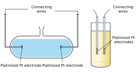
A conductivity cell (shown in the accompanying figure card, available in a couple of common designs) essentially consists of two platinized platinum electrodes — platinum coated electrochemically with a fine deposit of platinum black — held a fixed distance $l$ apart, each with cross-sectional area $A$ .

Figure 2.4Two different types of conductivity cells.

Fig. 2.4 — Two different types of conductivity cells.

Drawn by us to help you understand the concept clearly, and verified to make sure it's accurate. For exams, practice from your NCERT textbook's own diagram.

Figure 2.4 shows two common designs of a conductivity cell used to measure the resistance (and hence conductivity) of an electrolyte solution.

Left panel: A horizontal cylindrical glass vessel, partially filled with the solution. Two platinized platinum electrodes (coated with finely divided platinum black) enter through the vessel's two upright side arms and are immersed in the solution. Connecting wires extend upward from the side arms.
Right panel: A vertical cylindrical vessel holding the solution, with the same pair of platinized platinum electrodes and connecting wires.

The key physical idea is that the solution confined between the two electrodes behaves like a conducting column of length $l$ and uniform cross-sectional area $A$ . The resistance $R$ of this column is given by:

R = \rho \frac{l}{A} = \frac{1}{\kappa} \cdot \frac{l}{A}

where:

$\rho$ = resistivity of the solution (in $\Omega \, \text{m}$ )
$\kappa$ = conductivity of the solution (in $\text{S} \, \text{m}^{-1}$ ), with $\kappa = 1/\rho$
$l$ = distance between the electrodes (in m)
$A$ = area of cross-section of each electrode (in $\text{m}^2$ )

The ratio $\frac{l}{A}$ is called the cell constant, denoted by $G^*$ . It has dimensions of $\text{m}^{-1}$ (or $\text{cm}^{-1}$ ). Because $l$ and $A$ are difficult to measure accurately, the cell constant is determined experimentally using a solution of known conductivity (e.g., KCl solutions from Table 2.3). Once $G^*$ is known, the conductivity of any solution can be found from:

$\kappa = \frac{G^*}{R}$ …

The solution confined between them behaves as a column of length $l$ and area $A$ , so its resistance follows the same relation used for any conducting column:

R = \rho\,\frac{l}{A} = \frac{l}{\kappa A}

Cell Constant

Because measuring $l$ and $A$ directly for a real cell is inconvenient and unreliable, the ratio $l/A$ is instead determined experimentally and called the cell constant, $G^*$ :

G^{*} = \frac{l}{A} = R\,\kappa

$G^*$ — cell constant, with dimensions of (length)⁻¹; depends only on the cell's geometry (electrode spacing and area)

The usual way to find $G^*$ is to fill the cell with a solution whose conductivity is already known precisely at various concentrations and temperatures — KCl solutions are the standard choice for this — and measure the cell's resistance with that solution inside. A reference data table of the conductivity and molar conductivity of KCl solutions at known concentrations is provided as a separate card for exactly this purpose; it is not reproduced here.

Table 2.3Conductivity and Molar conductivity of KCl solutions at 298.15K

Concentration (mol L⁻¹)	Concentration (mol m⁻³)	Conductivity (S cm⁻¹)	Conductivity (S m⁻¹)	Molar Conductivity (S cm² mol⁻¹)	Molar Conductivity (S m² mol⁻¹)
1.000	1000	0.1113	11.13	111.3	$111.3\times10^{-4}$
0.100	100.0	0.0129	1.29	129.0	$129.0\times10^{-4}$

Measuring an Unknown Solution's Resistance

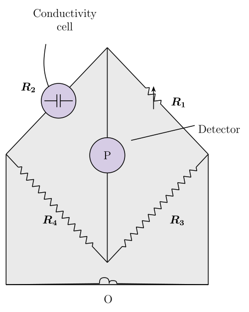
Once the cell constant is known, the same cell can be used to find the resistance (and hence conductivity) of any other solution. The measurement arrangement (shown in the accompanying figure card) is a modified Wheatstone-bridge circuit: two fixed resistances, a variable resistance, and the conductivity cell itself (carrying the unknown resistance) are wired into the four arms of the bridge, which is fed by the AC oscillator and balanced using a suitable detector (such as a headphone) so that no current flows through the detector arm.

Figure 2.5Arrangement for measurement of resistance of a solution of an electrolyte.

Fig. 2.5 — Arrangement for measurement of resistance of a solution of an electrolyte.

Drawn by us to help you understand the concept clearly, and verified to make sure it's accurate. For exams, practice from your NCERT textbook's own diagram.

What the Figure Shows

The figure is a schematic of a Wheatstone bridge circuit, drawn as a diamond-shaped network of four resistors. An oscillator (O) — an AC source in the audio frequency range (550–5000 Hz) — feeds the bridge at two opposite corners. A detector (P) — typically a headphone or electronic null detector — is placed across the other two corners. The four arms of the bridge contain:

$R_1$ : a variable resistance (adjustable)
$R_3$ and $R_4$ : two fixed resistances of known values
$R_2$ : the unknown resistance of the solution in the conductivity cell

The bridge is balanced when the detector shows zero current. At balance, the unknown resistance is given by:

R_2 = \frac{R_1 R_4}{R_3}

Physical Idea Behind the Measurement

The goal is to measure the resistance of an electrolyte solution without using direct current (DC), which would cause electrolysis and change the solution. An alternating current (AC) from the oscillator avoids this. The Wheatstone bridge method compares the unknown resistance $R_2$ with known resistances $R_1$ , $R_3$ , $R_4$ under AC conditions. Once $R_2$ is found, the conductivity $\kappa$ (the reciprocal of resistivity) is obtained using the cell constant $G^*$ :

\kappa = \frac{G^*}{R_2}

where $G^* = \frac{l}{A}$ (distance between electrodes divided by their area). The cell constant is determined beforehand using a standard KCl solution of known conductivity.

Key Formulas Developed from This Figure

Resistance of a solution column (from the geometry of the conductivity cell):

R = \rho \frac{l}{A} = \frac{1}{\kappa} \cdot \frac{l}{A}

$R$ = resistance (ohm, $\Omega$ )
$\rho$ = resistivity ( $\Omega$ m)
$\kappa$ = conductivity (S m $^{-1}$ )
$l$ = distance between electrodes (m)
$A$ = cross-sectional area of electrodes (m $^2$ )

Cell constant:

G^* = \frac{l}{A} = R \kappa

$G^*$ has units of m $^{-1}$ (or cm $^{-1}$ )

Wheatstone bridge balance condition:

R_2 = \frac{R_1 R_4}{R_3}

$R_2$ = unknown resistance of the solution
$R_1$ = variable resistance
$R_3$ , $R_4$ = fixed resistances

Conductivity from measured resistance:

$\kappa = \frac{G^*}{R_2}$ …

Under balance, the unknown resistance of the solution can be read off directly from the known bridge resistances.

Many modern conductivity meters skip this arithmetic and directly display the conductance or resistance of the solution in the cell. Either way, once the cell constant and the measured resistance $R$ are both known, the conductivity of the solution follows from:

\kappa = \frac{\text{cell constant}}{R} = \frac{G^{*}}{R}

The conductivity of solutions of different electrolytes in the same solvent, at the same temperature, differs because of differences in the charge and size of the ions produced, and how easily those ions move under a potential gradient. Comparing $\kappa$ values alone across electrolytes is therefore not very meaningful — a fairer comparison needs a quantity that also accounts for how much electrolyte is actually present in solution.

Molar Conductivity

This more meaningful quantity is called molar conductivity, denoted $\Lambda_m$ (Greek, lambda). It relates the conductivity of a solution to its concentration:

\Lambda_m = \frac{\kappa}{c}

$\Lambda_m$ — molar conductivity

$\kappa$ — conductivity of the solution

$c$ — molar concentration of the electrolyte

Units and the factor of 1000. If $\kappa$ is expressed in S m⁻¹ and $c$ in mol m⁻³, then $\Lambda_m$ comes out directly in S m² mol⁻¹. In practice, though, concentration is usually quoted as molarity (mol L⁻¹), and since

1\ \text{mol m}^{-3} = 1000\ (\text{L/m}^3) \times \text{molarity (mol/L)}

a conversion factor of 1000 has to be carried through the calculation whenever molarity in mol L⁻¹ is combined with a conductivity expressed per centimetre or per metre. Concretely, if $\kappa$ is in S cm⁻¹ and concentration is molarity in mol L⁻¹:

$\Lambda_m\,(\text{S cm}^2\,\text{mol}^{-1}) = \frac{\kappa\,(\text{S cm}^{-1}) \times 1000\,(\text{cm}^3/\text{L})}{\text{molarity (mol L}^{-1})}$ …

Start your 14-day free trial to unlock the full solution →

← Previous · 2.4Conductance of Electrolytic Solutions Next · 2.4.1 →Example 2.4 — Resistance of a conductivity cell filled with 0.1molL⁻¹ KCl solution i…