Chemistry · Ch 6 — Equilibrium

Equilibrium in Chemical Processes – Dynamic Equilibrium

6.2

Equilibrium in Chemical Processes – Dynamic Equilibrium

Chemical reactions, like physical processes, can reach a state of equilibrium. The key difference is that chemical equilibrium involves the transformation of substances into different chemical species, not just a change in physical state.

The Nature of Chemical Equilibrium

Consider a general reversible reaction:

A + B \rightleftharpoons C + D

When reactants A and B are mixed, the forward reaction (A + B → C + D) begins. As products C and D accumulate, the reverse reaction (C + D → A + B) starts and gradually speeds up. Meanwhile, the forward reaction slows down because the concentrations of A and B are decreasing.

Eventually, the rates of the forward and reverse reactions become equal. At this point, the concentrations of all species — reactants and products — stop changing and remain constant over time. This is the state of chemical equilibrium.

Figure 6.2Attainment of chemical equilibrium.

Fig. 6.2 — Attainment of chemical equilibrium.

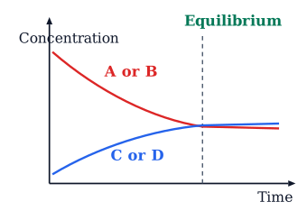
Drawn by us to help you understand the concept clearly, and verified to make sure it's accurate. For exams, practice from your NCERT textbook's own diagram.

What Fig. 6.2 Actually Shows

The figure is a concentration-versus-time graph. The horizontal axis is time, increasing to the right. The vertical axis is concentration (in mol L $^{-1}$ ). Two curves are plotted on the same set of axes.

One curve, labelled "A or B" and drawn in red, starts at a high concentration on the vertical axis and falls steeply at first, then more gradually, until it becomes a flat horizontal line. This represents the concentration of a reactant (either A or B, since in the reaction A + B $\rightleftharpoons$ C + D the two reactants are consumed in the same proportion if they start in stoichiometric ratio). The other curve, labelled "C or D" and drawn in blue, starts at zero concentration on the vertical axis and rises steeply at first, then more gradually, until it too becomes a flat horizontal line. This represents the concentration of a product (either C or D).

A vertical dashed line is drawn at the time when both curves become flat. This line is labelled "Equilibrium". To the left of this line, the curves are changing; to the right, they are constant.

The Physical Idea

The graph teaches the central fact about chemical equilibrium: it is a state reached over time, not an instantaneous event. When reactants A and B are first mixed, their concentration is high, so the forward reaction (A + B $\rightarrow$ C + D) is fast. Products C and D are absent, so the reverse reaction (C + D $\rightarrow$ A + B) cannot occur at all. As time passes, the forward reaction consumes A and B, so their concentration falls. This slows the forward reaction. Meanwhile, C and D accumulate, so the reverse reaction begins and gradually speeds up.

The two rates approach each other. When they become exactly equal, the concentrations stop changing. The curves become flat. This is equilibrium.

Important

The flat lines do not mean the reactions have stopped. They mean the forward and reverse reactions are proceeding at the same rate, so there is no net change in concentration. This is dynamic equilibrium, not static equilibrium.

The textbook emphasises that the same equilibrium state can be reached from the opposite direction — starting with only C and D, the curves would be reversed (C and D falling, A and B rising) but they would level off at the same final concentrations.

The Key Formula Developed from This Figure

The figure motivates the law of chemical equilibrium. For the general reaction

a\text{A} + b\text{B} \rightleftharpoons c\text{C} + d\text{D}

the equilibrium constant $K_c$ is defined as

K_c = \frac{[\text{C}]^c [\text{D}]^d}{[\text{A}]^a [\text{B}]^b}

where each symbol in square brackets means the equilibrium concentration of that species (in mol L $^{-1}$ ), and the exponents are the stoichiometric coefficients from the balanced equation.

For the specific reaction shown in the figure, A + B $\rightleftharpoons$ C + D, this becomes

$K_c = \frac{[\text{C}][\text{D}]}{[\text{A}][\text{B}]}$ …

Important

At chemical equilibrium, the rates of the forward and reverse reactions are equal, but the concentrations of reactants and products are constant — not necessarily equal to each other.

Dynamic Nature of Equilibrium

Chemical equilibrium is dynamic, not static. The forward and reverse reactions continue to occur at equal rates, so there is constant interconversion between reactants and products. No net change in composition is observed because the two opposing processes cancel each other out.

Demonstration Using Isotopes: Haber's Process

The dynamic nature of equilibrium was elegantly demonstrated in the synthesis of ammonia:

N_2(g) + 3H_2(g) \rightleftharpoons 2NH_3(g)

Fritz Haber conducted experiments where he started with known amounts of $N_2$ and $H_2$ at high temperature and pressure.

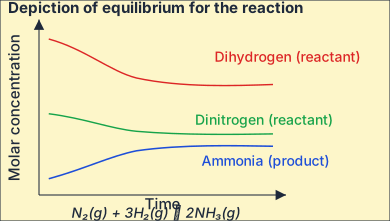
Figure 6.4Depiction of equilibrium for the reaction N₂(g) + 3H₂(g) ⇌ 2NH₃(g)

Fig. 6.4 — Depiction of equilibrium for the reaction N₂(g) + 3H₂(g) ⇌ 2NH₃(g)

Drawn by us to help you understand the concept clearly, and verified to make sure it's accurate. For exams, practice from your NCERT textbook's own diagram.

The figure is a concentration-versus-time graph for the reaction N₂(g) + 3H₂(g) ⇌ 2NH₃(g), showing the reaction approaching and reaching equilibrium.

Three curves are plotted. Dihydrogen (reactant) starts at a relatively high concentration and falls as it's consumed, then levels off once equilibrium is reached. Dinitrogen (reactant) starts lower and follows the same shape — it also falls and levels off, but by a smaller amount (only one N₂ is consumed for every three H₂, matching the reaction's 3:1 stoichiometry). Ammonia (product) starts at zero, since none exists before the reaction begins, and rises steadily until it too levels off. …

He measured the concentrations of $NH_3$ , unreacted $N_2$ , and unreacted $H_2$ at regular intervals. After a certain time, the composition of the mixture became constant — equilibrium was reached.

To prove the reaction was still occurring, Haber repeated the experiment using deuterium ( $D_2$ ) instead of ordinary hydrogen ( $H_2$ ). The reaction mixtures starting with either $H_2$ or $D_2$ reached equilibrium with the same composition, except that $D_2$ and $ND_3$ were present instead of $H_2$ and $NH_3$ .

The critical test came when these two equilibrium mixtures were combined and left for a while. Analysis using a mass spectrometer revealed the presence of all deuterium-containing forms of ammonia ( $NH_3$ , $NH_2D$ , $NHD_2$ , $ND_3$ ) and all forms of dihydrogen ( $H_2$ , $HD$ , $D_2$ ). This scrambling of hydrogen and deuterium atoms could only happen if the forward and reverse reactions were continuing in the mixture. If the reaction had stopped at equilibrium, no mixing of isotopes would have occurred.

Try it yourself: a classroom demonstration of dynamic equilibrium. You don't need radioactive or isotope-labelled material to see this idea in action -- a simple two-cylinder demonstration works with a group of 5-6 students. Take two 100 mL measuring cylinders (labelled 1 and 2) and two glass tubes about 30 cm long. Half-fill cylinder 1 with coloured water (a crystal of potassium permanganate works well) and leave cylinder 2 empty. Put one tube in each cylinder. Using the tube in cylinder 1, transfer some coloured water down into cylinder 2; using the tube in cylinder 2, transfer some water back into cylinder 1. Keep repeating both transfers, back and forth, and watch the water level in each cylinder. Eventually the two levels stop changing -- but if you keep transferring water anyway, the levels stay exactly where they were. That's the whole point: the transfers never actually stopped, they just became equal in both directions, so there's no more net change. If you repeat the experiment with two tubes of different diameters, the final levels in the two cylinders come out unequal -- a reminder that at real chemical equilibrium the forward and reverse rates are equal, not necessarily the concentrations themselves.

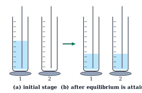
Figure 6.3Demonstrating the dynamic nature of equilibrium.

Fig. 6.3 — Demonstrating the dynamic nature of equilibrium.

Drawn by us to help you understand the concept clearly, and verified to make sure it's accurate. For exams, practice from your NCERT textbook's own diagram.

Fig. 6.3 is a simple two-panel diagram that uses a physical analogy to make the abstract idea of dynamic equilibrium concrete. The figure shows two 100 mL measuring cylinders, labelled 1 and 2, with two glass tubes (one in each cylinder). In panel (a), labelled “initial stage”, cylinder 1 is nearly half-filled with coloured water (representing a high concentration of reactant) and cylinder 2 is empty (representing zero product). In panel (b), labelled “final stage after the equilibrium is attained”, the coloured water is equally distributed between the two cylinders — both show the same level of liquid.

The key teaching point is that even after the levels become constant, the transfer of water continues. The two tubes are used to repeatedly move small amounts of water back and forth: one tube transfers water from cylinder 1 to cylinder 2, the other from cylinder 2 to cylinder 1. At the start, the net flow is from the full cylinder to the empty one. As the levels approach equality, the rate of transfer from 1 to 2 decreases (less water in cylinder 1 to pick up) and the rate from 2 to 1 increases (more water in cylinder 2). When the two transfer rates become equal, the levels stop changing — but the individual transfers never stop. This is the dynamic equilibrium: a steady state maintained by two opposing processes occurring at the same rate.

The textbook then draws the analogy explicitly: the “level” of coloured water corresponds to the concentration of reactants and products. Cylinder 1 is like the reactant side, cylinder 2 like the product side. The constant level at equilibrium corresponds to constant concentrations. The fact that water keeps moving even after the levels are steady mirrors the fact that, at chemical equilibrium, the forward and reverse reactions continue to occur — they do not stop — but their rates are equal, so there is no net change in composition.

Note

A subtle but important detail: if the two glass tubes have different diameters, the equilibrium levels in the two cylinders will be different. This is because a wider tube transfers more water per dip, so the rates balance at a different height. In chemical terms, this corresponds to the fact that the equilibrium constant depends on the stoichiometric coefficients — the “diameters” of the forward and reverse pathways are not necessarily equal.

The figure directly sets up the central quantitative idea of the chapter: for a reversible reaction $a\text{A} + b\text{B} \rightleftharpoons c\text{C} + d\text{D}$ , at equilibrium the rates of the forward and reverse reactions are equal, and the concentrations obey the law of chemical equilibrium:

K_c = \frac{[\text{C}]^c [\text{D}]^d}{[\text{A}]^a [\text{B}]^b}

Note

The isotope experiment proves that equilibrium is not a static condition where reactions stop. Instead, it is a dynamic balance where forward and reverse reactions proceed at equal rates, constantly exchanging atoms between reactants and products.

Equilibrium Can Be Reached from Either Direction

A crucial feature of chemical equilibrium is that the same equilibrium state can be reached regardless of whether we start with pure reactants or pure products.

Consider the reaction:

$H_2(g) + I_2(g) \rightleftharpoons 2HI(g)$ …

Figure 6.5Chemical equilibrium in the reaction H₂(g) + I₂(g) ⇌ 2HI(g) can be attained from either direction.

Fig. 6.5 — Chemical equilibrium in the reaction H₂(g) + I₂(g) ⇌ 2HI(g) can be attained from either direction.

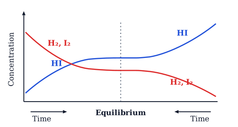
Drawn by us to help you understand the concept clearly, and verified to make sure it's accurate. For exams, practice from your NCERT textbook's own diagram.

The figure is a concentration-versus-time graph for the reaction $\text{H}_2(g) + \text{I}_2(g) \rightleftharpoons 2\text{HI}(g)$ . The vertical axis is concentration (in mol/L), and the horizontal axis is time (in seconds or minutes). A vertical dashed line labelled Equilibrium divides the plot into two halves.

On the left side of the equilibrium line, the graph shows the system starting with only $\text{H}_2$ and $\text{I}_2$ (both shown in red). Their concentrations are initially high and then fall smoothly as the forward reaction consumes them. Meanwhile, the concentration of $\text{HI}$ (shown in blue) starts at zero and rises. The curves are mirror-like: as one red curve drops, the blue curve climbs. Eventually, all three curves become horizontal — they stop changing. That flat region, just before the vertical equilibrium line, is the equilibrium state reached from the reactant side.

On the right side of the equilibrium line, the graph shows the reverse experiment. Here the system starts with only $\text{HI}$ (blue curve high, red curves at zero). As time passes, $\text{HI}$ decomposes — its blue curve falls — while $\text{H}_2$ and $\text{I}_2$ appear and rise. Again, after some time, all three curves flatten out. The critical point: the flat horizontal values on the right side are exactly the same as those on the left side. The equilibrium concentrations of $\text{H}_2$ , $\text{I}_2$ , and $\text{HI}$ are identical regardless of whether you started from pure reactants or pure product.

Important

The figure demonstrates that chemical equilibrium is a dynamic state reached from either direction. The equilibrium concentrations are fixed by the reaction conditions (temperature, pressure) and do not depend on the starting composition.

The textbook uses this figure to introduce the Law of Chemical Equilibrium and the equilibrium constant expression. For the reaction

a\text{A} + b\text{B} \rightleftharpoons c\text{C} + d\text{D}

at equilibrium, the ratio

K_c = \frac{[\text{C}]^c [\text{D}]^d}{[\text{A}]^a [\text{B}]^b}

is constant at a given temperature. For the specific reaction in the figure,

K_c = \frac{[\text{HI}]^2}{[\text{H}_2][\text{I}_2]}

where $[\text{HI}]$ , $[\text{H}_2]$ , and $[\text{I}_2]$ are the equilibrium concentrations (in mol/L) read from the flat portions of the graph. The fact that the same $K_c$ value is obtained from both sides of the figure is the experimental basis for the law. …

Start your 14-day free trial to unlock the full solution →

← Previous · 6.1.5General Characteristics of Equilibria Involving Physical Processes Next · 6.3 →Law of Chemical Equilibrium and Equilibrium Constant