Mathematics · Ch 10 — Vector Algebra

Components of a Vector

10.5.1

Components of a Vector

Introducing the Component Form of a Vector

To calculate with vectors precisely, we describe any vector by numbers — its components along the coordinate axes. We first define the three unit vectors along the axes.

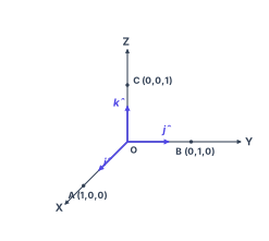
Consider the points $A(1,0,0)$ , $B(0,1,0)$ , and $C(0,0,1)$ on the $x$ , $y$ , and $z$ -axes. The vectors $\overrightarrow{OA}$ , $\overrightarrow{OB}$ , $\overrightarrow{OC}$ each have magnitude 1 and are the unit vectors along the axes $OX$ , $OY$ , $OZ$ , denoted $\hat{i}$ , $\hat{j}$ , $\hat{k}$ .

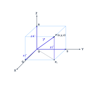
Take any point $P(x, y, z)$ , and let $P_1$ be the foot of the perpendicular from $P$ onto the $XOY$ plane. Then:

$\overrightarrow{OP_1} = x\hat{i} + y\hat{j}$ (since $P_1 = (x, y, 0)$ ),
$\overrightarrow{P_1P} = z\hat{k}$ .

Therefore the position vector of $P$ with respect to the origin $O$ is:

\overrightarrow{OP} = \overrightarrow{OP_1} + \overrightarrow{P_1P} = x\hat{i} + y\hat{j} + z\hat{k}

This is the component form of $\vec{r} = \overrightarrow{OP}$ .

$x$ , $y$ , $z$ are the scalar components (rectangular components) of $\vec{r}$ .
$x\hat{i}$ , $y\hat{j}$ , $z\hat{k}$ are the vector components of $\vec{r}$ along the respective axes.

Note

The scalar components $x$ , $y$ , $z$ are simply the coordinates of $P$ . The component form directly links a vector to the coordinates of its terminal point when its initial point is at the origin.

Magnitude of a Vector in Component Form

Applying the Pythagoras theorem twice: in the right triangle $OQP_1$ , $|\overrightarrow{OP_1}| = \sqrt{x^2 + y^2}$ ; then in the right triangle $OP_1P$ with $|\overrightarrow{P_1P}| = |z|$ :

|\vec{r}| = \sqrt{x^2 + y^2 + z^2}

|\vec{r}| = \sqrt{x^2 + y^2 + z^2}

Operations on Vectors in Component Form

Let $\vec{a} = a_1\hat{i} + a_2\hat{j} + a_3\hat{k}$ and $\vec{b} = b_1\hat{i} + b_2\hat{j} + b_3\hat{k}$ . The operations are defined component-wise.

(i) Addition of Vectors

\vec{a} + \vec{b} = (a_1 + b_1)\hat{i} + (a_2 + b_2)\hat{j} + (a_3 + b_3)\hat{k}

(ii) Subtraction of Vectors

\vec{a} - \vec{b} = (a_1 - b_1)\hat{i} + (a_2 - b_2)\hat{j} + (a_3 - b_3)\hat{k}

(iii) Equality of Vectors

\vec{a} = \vec{b} \iff a_1 = b_1, \quad a_2 = b_2, \quad a_3 = b_3

(iv) Multiplication of a Vector by a Scalar

\lambda\vec{a} = (\lambda a_1)\hat{i} + (\lambda a_2)\hat{j} + (\lambda a_3)\hat{k}

Distributive Laws for Scalar Multiplication

Let $\vec{a}$ and $\vec{b}$ be any two vectors, and $k$ and $m$ any scalars.

›Proof

Proof of Distributive Laws

Law (i): $k(\vec{a} + \vec{b}) = k\vec{a} + k\vec{b}$

$k(\vec{a} + \vec{b}) = k(a_1+b_1)\hat{i} + k(a_2+b_2)\hat{j} + k(a_3+b_3)\hat{k}$

$= (ka_1 + kb_1)\hat{i} + (ka_2 + kb_2)\hat{j} + (ka_3 + kb_3)\hat{k}$

$= (ka_1\hat{i} + ka_2\hat{j} + ka_3\hat{k}) + (kb_1\hat{i} + kb_2\hat{j} + kb_3\hat{k}) = k\vec{a} + k\vec{b}$ .

Law (ii): $(k+m)\vec{a} = k\vec{a} + m\vec{a}$

$(k+m)\vec{a} = (k+m)a_1\hat{i} + (k+m)a_2\hat{j} + (k+m)a_3\hat{k}$

$= (ka_1 + ma_1)\hat{i} + (ka_2 + ma_2)\hat{j} + (ka_3 + ma_3)\hat{k}$

$= (ka_1\hat{i} + ka_2\hat{j} + ka_3\hat{k}) + (ma_1\hat{i} + ma_2\hat{j} + ma_3\hat{k}) = k\vec{a} + m\vec{a}$ .

Collinearity of Vectors in Component Form

Two vectors $\vec{a}$ and $\vec{b}$ are collinear (parallel) if and only if there exists a non-zero scalar $\lambda$ such that $\vec{b} = \lambda\vec{a}$ . In components:

b_1 = \lambda a_1, \quad b_2 = \lambda a_2, \quad b_3 = \lambda a_3

so the ratios of corresponding components are equal:

$\frac{b_1}{a_1} = \frac{b_2}{a_2} = \frac{b_3}{a_3} = \lambda$ …

Figure 10.13The unit vectors i-hat, j-hat and k-hat along the X, Y and Z axes from origin O, reaching points A(1,0,0), B(0,1,0) and C(0,0,1).

Fig. 10.13 — The unit vectors i-hat, j-hat and k-hat along the X, Y and Z axes from origin O, reaching points A(1,0,0), B(0,1,0) and C(0,0,1).

Drawn by us to help you understand the concept clearly, and verified to make sure it's accurate. For exams, practice from your NCERT textbook's own diagram.

Fig 10.13 is the foundational picture for the entire component form of vectors in three dimensions. It shows a standard right-handed 3D coordinate system with the origin at O. The X-axis runs to the lower-left, the Y-axis to the right, and the Z-axis straight up. Along each positive axis, a short indigo arrow is drawn: these are the three unit vectors $\hat{i}$ (along X), $\hat{j}$ (along Y), and $\hat{k}$ (along Z). Three specific points are marked on the axes: A at $(1,0,0)$ on the X-axis, B at $(0,1,0)$ on the Y-axis, and C at $(0,0,1)$ on the Z-axis.

The entire purpose of this figure is to give you a visual anchor for the idea that any vector in space can be built from three perpendicular building blocks. The vectors $\overrightarrow{OA}$ , $\overrightarrow{OB}$ , and $\overrightarrow{OC}$ each have length exactly 1 — they are the unit vectors along the axes. The textbook names them $\hat{i}$ , $\hat{j}$ , $\hat{k}$ respectively. Once you accept that these three arrows exist, you can represent any point $P(x,y,z)$ by walking from O to P using a combination of them: go $x$ units along $\hat{i}$ , then $y$ units along $\hat{j}$ , then $z$ units along $\hat{k}$ .

Important

The figure directly leads to the component form of a position vector. For any point $P(x,y,z)$ , its position vector $\vec{r} = \overrightarrow{OP}$ is written as

$\vec{r} = x\hat{i} + y\hat{j} + z\hat{k}$

Here $x$ , $y$ , $z$ are the scalar components (the actual numbers), and $x\hat{i}$ , $y\hat{j}$ , $z\hat{k}$ are the vector components along the respective axes.

The figure also sets up the geometry for finding the magnitude (length) of any vector. Look at the right triangle formed in the XOY plane: from O to $P_1$ (the foot of the perpendicular from P onto the XOY plane), the distance is $\sqrt{x^2 + y^2}$ . Then, in the vertical right triangle from $P_1$ to P, the height is $z$ . Applying Pythagoras twice gives the famous result: …

Figure 10.14Position vector OP = r resolved into rectangular components x i-hat, y j-hat and z k-hat as the edges of a cuboid, with P1 the foot of the perpendicular from P onto the XY-plane.

Fig. 10.14 — Position vector OP = r resolved into rectangular components x i-hat, y j-hat and z k-hat as the edges of a cuboid, with P1 the foot of the perpendicular from P onto the XY-plane.

Drawn by us to help you understand the concept clearly, and verified to make sure it's accurate. For exams, practice from your NCERT textbook's own diagram.

Fig 10.14 is the central geometric picture that connects the coordinates of a point in 3D space to the vector representation of its position. It shows a rectangular box (a cuboid) with one corner at the origin O and the opposite corner at the point P(x, y, z). The three edges of the cuboid that meet at O lie along the positive x‑axis, y‑axis, and z‑axis, respectively.

The key construction is the foot of the perpendicular from P onto the XY‑plane. That point is labelled P₁. The line OP₁ is drawn as a dotted diagonal across the base of the cuboid (the rectangle in the XY‑plane), and the vertical segment P₁P is drawn solid, parallel to the z‑axis. So the position vector $\vec{r} = \overrightarrow{OP}$ is the space diagonal of the cuboid, and it is broken into three mutually perpendicular components: one along the x‑axis (from O to Q, labelled $x\hat{i}$ ), one along the y‑axis (from O to S, labelled $y\hat{j}$ ), and one along the z‑axis (from O to R, labelled $z\hat{k}$ ). The points Q, S, and R are the projections of P onto the x‑axis, y‑axis, and z‑axis, respectively.

The physical idea is that any vector in 3D space can be expressed as the sum of three independent, perpendicular pieces — one for each coordinate direction. The figure makes this decomposition visible: you can see that $\overrightarrow{OP} = \overrightarrow{OQ} + \overrightarrow{OS} + \overrightarrow{OR}$ , which in vector notation becomes

\vec{r} = x\hat{i} + y\hat{j} + z\hat{k}.

Here $x$ , $y$ , $z$ are the scalar components (the coordinates of P), and $\hat{i}$ , $\hat{j}$ , $\hat{k}$ are the unit vectors along the axes.

The textbook uses this figure to derive the formula for the magnitude (length) of a vector. In the right‑angled triangle OQP₁ (lying in the XY‑plane), the diagonal OP₁ has length $\sqrt{x^2 + y^2}$ . Then in the vertical right‑angled triangle OP₁P, with legs OP₁ and P₁P = z, the hypotenuse OP gives

|\vec{r}| = \sqrt{(\sqrt{x^2 + y^2})^2 + z^2} = \sqrt{x^2 + y^2 + z^2}.

|\vec{r}| = \sqrt{x^2 + y^2 + z^2}

This is the 3D version of the Pythagorean theorem, and it is the single most important formula that Fig 10.14 is designed to teach. Every symbol is defined by the geometry of the cuboid: $x$ , $y$ , $z$ are the lengths of the three edges meeting at O, and the magnitude $|\vec{r}|$ is the length of the space diagonal. …

Start your 14-day free trial to unlock the full solution →

← Previous · 10.5Multiplication of a Vector by a Scalar Next · 10.5.1 →Example 4 — Find the values of x, y and z so that the vectors veca=xhati+2hatj+zha…