Economics · Ch 9 — Determination of Income and Employment

Effect of an Autonomous Change in Aggregate Demand on Income

9.3.2

Effect of an Autonomous Change in Aggregate Demand on Income

4.3.2 Effect of an Autonomous Change in Aggregate Demand on Income and Output

The equilibrium level of income is determined by aggregate demand. If aggregate demand changes, the equilibrium level of income must change as well. This change in aggregate demand can originate from any of its components.

Sources of Change in Aggregate Demand

Aggregate demand can shift due to changes in either consumption or investment.

Change in consumption can happen for two reasons:

A change in autonomous consumption ( $\bar{C}$ ) — the part of consumption that does not depend on income.
A change in the marginal propensity to consume ( $c$ ) — the fraction of each additional rupee of income that is spent on consumption.

Change in investment requires more careful attention. We have assumed so far that investment is autonomous — meaning it does not depend on income. But autonomous does not mean fixed forever. Investment depends on several factors other than income:

Availability of credit: When credit is easily available, firms are more likely to borrow and invest.
Interest rate: The interest rate is the cost of investible funds. At higher interest rates, firms tend to lower their investment because borrowing becomes more expensive.

Let us now focus on what happens when investment changes, using a concrete numerical example.

A Numerical Example

Suppose the consumption function is:

C = 40 + 0.8Y

and autonomous investment is $I = 10$ .

In this case, aggregate demand is:

AD = C + I = 40 + 0.8Y + 10 = 50 + 0.8Y

Equilibrium requires that aggregate demand equals aggregate supply (output $Y$ ):

Y = 50 + 0.8Y

Y - 0.8Y = 50

0.2Y = 50

Y = \frac{50}{0.2} = 250

So the initial equilibrium income is 250.

Now suppose investment rises to $I = 20$ . The new aggregate demand becomes:

AD = 40 + 0.8Y + 20 = 60 + 0.8Y

Setting $Y = AD$ :

Y = 60 + 0.8Y

0.2Y = 60

Y = \frac{60}{0.2} = 300

The new equilibrium income is 300.

Watch out

Notice that investment increased by 10 (from 10 to 20), but income increased by 50 (from 250 to 300). The increase in income is five times the increase in investment. This is not a coincidence — it is the working of the multiplier, which we will examine in detail in section 4.3.3.

Graphical Representation

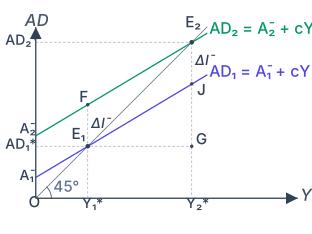
The graph (Fig. 4.7 in the textbook) uses the 45° line diagram. The 45° line represents all points where aggregate demand equals aggregate supply ( $Y = AD$ ).

Figure 4.7Equilibrium Output and Aggregate Demand in the Fixed Price Model

Fig. 4.7 — Equilibrium Output and Aggregate Demand in the Fixed Price Model

Drawn by us to help you understand the concept clearly, and verified to make sure it's accurate. For exams, practice from your textbook's own diagram.

Fig. 4.7 shows how an autonomous increase in expenditure raises equilibrium output by a multiplied amount in the fixed-price model. The vertical axis is Aggregate Demand ( $AD$ ) and the horizontal axis is income $Y$ ; a $45^\circ$ line from the origin marks all points where $AD = Y$ .

Two parallel, upward-sloping aggregate demand lines are drawn, both with slope equal to the marginal propensity to consume $c$ :

the initial line $AD_1 = \bar{A}_1 + cY$ , with the lower vertical intercept $\bar{A}_1$ ;
the shifted line $AD_2 = \bar{A}_2 + cY$ , with the higher intercept $\bar{A}_2$ .

An increase in autonomous expenditure ( $\Delta\bar{I} = \bar{A}_2 - \bar{A}_1$ ) lifts the whole line upward in parallel from $AD_1$ to $AD_2$ (the slope is unchanged because $c$ has not changed).

Initially the economy is in equilibrium at $E_1$ , where $AD_1$ meets the $45^\circ$ line, giving output $Y_1^{*}$ . At this same output the new line $AD_2$ lies above $E_1$ at point F; the gap $E_1F$ is the initial injection of autonomous expenditure, $\Delta\bar{I} = E_1F = E_2J$ . Because demand now exceeds output, firms expand production until the new equilibrium $E_2$ is reached where $AD_2$ cuts the $45^\circ$ line, giving the higher output $Y_2^{*}$ .

Important

The total rise in output, $E_1G = E_2G$ , is larger than the initial increment $\Delta\bar{I} = E_1F$ . This is the multiplier: an autonomous change in spending changes equilibrium income by a larger amount,

$\Delta Y = \frac{1}{1-c}\,\Delta\bar{A}.$ …

The initial aggregate demand line $AD_1$ has the equation $AD_1 = 50 + 0.8Y$ . It intersects the 45° line at point $E_1$ , giving equilibrium output $Y_1^* = 250$ .

When investment increases, the aggregate demand line shifts upward in a parallel fashion to $AD_2$ , with equation $AD_2 = 60 + 0.8Y$ . The slope remains the same (0.8) because the marginal propensity to consume has not changed — only the intercept has increased.

At the old equilibrium output $Y_1^* = 250$ , the new aggregate demand is:

AD_2 = 60 + 0.8(250) = 60 + 200 = 260

The value of output at $Y_1^*$ is still 250. So aggregate demand (260) exceeds output (250) by an amount equal to 10. This excess demand is the distance $E_1F$ in the diagram — it represents the initial increment in autonomous expenditure ( $\Delta I = 10$ ).

Because of this excess demand, firms find their inventories depleting. They respond by increasing production. But as output rises, income rises, and consumption rises further (because $C = 40 + 0.8Y$ ). This creates additional demand, which calls forth additional output, and so on.

The new equilibrium is at point $E_2$ , where $AD_2$ intersects the 45° line. The new equilibrium output is $Y_2^* = 300$ , and the new equilibrium aggregate demand is $AD_2^* = 300$ .

Important

The total increase in output ( $\Delta Y = 50$ ) is greater than the initial increase in autonomous expenditure ( $\Delta I = 10$ ). The distance $E_1G = E_2G$ measures the total increase in output, while $E_1F = E_2J$ measures the initial increment in autonomous expenditure. The fact that $E_1G > E_1F$ shows that an initial change in autonomous expenditure has a multiplied effect on equilibrium income.

Algebraic Derivation of Equilibrium

We can derive the equilibrium condition in general terms.

Ex ante aggregate demand is:

AD = \bar{C} + cY + I

where $\bar{C}$ is autonomous consumption, $c$ is the marginal propensity to consume, and $I$ is autonomous investment.

Ex ante aggregate supply is simply $Y$ , the total output produced.

Equilibrium requires that the plans of suppliers are matched by the plans of those who provide final demand. Thus:

\bar{C} + cY + I = Y

Rearranging:

\bar{C} + I = Y - cY

\bar{C} + I = Y(1 - c)

Y = \frac{\bar{C} + I}{1 - c}

This is equation (4.4) in the textbook.

Y^* = \frac{\bar{C} + I}{1 - c}

where:

$Y^*$ is the equilibrium level of income
$\bar{C}$ is autonomous consumption
$I$ is autonomous investment
$c$ is the marginal propensity to consume ( $0 < c < 1$ )
$1 - c$ is the marginal propensity to save

The denominator $(1 - c)$ is crucial. Since $c$ is less than 1, $1 - c$ is a fraction, and dividing by a fraction yields a number larger than the numerator. This is the algebraic basis of the multiplier effect.

What Causes the Magnified Effect? …

Start your 14-day free trial to unlock the full solution →

← Previous · 9.3.1Macroeconomic Equilibrium with Price Level Fixed Next · 9.3.3 →The Multiplier Mechanism