Area Under Simple Curves

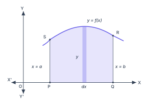
Fig 8.1 is the foundational picture for the entire chapter. It shows a standard Cartesian coordinate system with the x-axis labelled X'X and the y-axis labelled Y'Y, meeting at the origin O. In the first quadrant, a smooth, dome-shaped curve is drawn and labelled $y = f(x)$. Two vertical lines are drawn from the x-axis up to the curve: one at $x = a$ (meeting the curve at point S) and one at $x = b$ (meeting the curve at point R). The points where these vertical lines meet the x-axis are labelled P (at $x = a$) and Q (at $x = b$). The region bounded by the curve, the x-axis, and these two vertical lines is shaded indigo and labelled PQRS.

Inside this shaded region, a single very thin vertical strip is drawn. Its height is labelled $y$ (which is the value of $f(x)$ at that particular $x$), and its infinitesimal width is labelled $dx$. This strip is the key visual.

The physical idea this figure teaches is the method of vertical strips. The total area under the curve between $x = a$ and $x = b$ is not found in one go. Instead, you imagine slicing the region into an enormous number of these paper-thin vertical rectangles. The area of one such elementary strip is its height times its width: $dA = y \, dx = f(x) \, dx$. The total area $A$ is then the sum of the areas of all these strips from $x = a$ to $x = b$. In the language of calculus, this sum is the definite integral.

Here, $A$ is the total area of the shaded region. $y = f(x)$ is the height of the curve at any point $x$, and $dx$ is the infinitesimal width of each vertical strip. The limits $a$ and $b$ are the x-coordinates of the left and right boundaries of the region.

The figure also sets up the parallel idea for horizontal strips. If you rotate the picture so that the curve is expressed as $x = g(y)$, and the boundaries are horizontal lines $y = c$ and $y = d$, the area is given by $A = \int_c^d x \, dy = \int_c^d g(y) \, dy$. The textbook's Fig 8.2 illustrates this complementary view. …

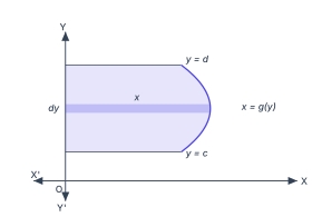
Fig 8.2 is the companion diagram to the formula for area using horizontal strips. It shows a Cartesian plane with the origin labelled O. The vertical axis is the y-axis, and the horizontal axis is the x-axis. A curve is drawn that bulges to the right — this is the graph of $x = g(y)$. The region of interest is bounded on the left by the y-axis itself, on the right by the curve $x = g(y)$, below by the horizontal line $y = c$, and above by the horizontal line $y = d$. The entire region is shaded in indigo.

The key visual element is a single horizontal elementary strip drawn inside the region. This strip runs from the y-axis (left boundary) to the curve (right boundary). Its length is labelled $x$ — that is, the $x$-coordinate of the curve at that particular $y$ value. Its thickness is labelled $dy$, an infinitesimally small change in $y$. The strip is horizontal because the boundaries on the left and right are functions of $y$, not of $x$.

The physical idea is straightforward: when a region is bounded on the left and right by curves expressed as $x = g(y)$, it is natural to slice it into thin horizontal strips rather than vertical ones. Each strip has area $dA = \text{length} \times \text{height} = x \cdot dy$. Adding up (integrating) these elementary areas from the bottom boundary $y = c$ to the top boundary $y = d$ gives the total area.

Here, $x = g(y)$ is the equation of the right-hand curve, $y = c$ is the lower limit, and $y = d$ is the upper limit. The variable of integration is $y$, and $dy$ is the thickness of each horizontal strip. This is the exact analogue of the vertical-strip formula $A = \int_a^b y \, dx$, but with the roles of $x$ and $y$ swapped. …

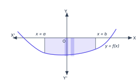
Fig 8.3 shows a curve $y = f(x)$ that crosses the $x$-axis three times. On the left, the curve lies above the $x$-axis, then it dips entirely below the axis between $x = a$ and $x = b$, and finally rises above the axis again on the right. The region between the curve and the $x$-axis over the interval $[a, b]$ — the part where the curve is below the axis — is shaded indigo. Inside that shaded region, two thin vertical elementary strips are drawn, each of height $|y|$ and width $dx$, to illustrate the idea of building the area from infinitesimally thin rectangles.

The physical idea this figure teaches is crucial: when a curve lies below the $x$-axis, the definite integral $\int_a^b f(x)\,dx$ gives a negative number because $f(x) < 0$ throughout the interval. But area is a positive quantity — we only care about the numerical magnitude. So the actual area of the region bounded by the curve, the $x$-axis, and the vertical lines $x = a$ and $x = b$ is taken as the absolute value:

Here, $f(x)$ is the height of the curve at a given $x$, $dx$ is the infinitesimal width of an elementary strip, and the integral sums the signed areas of all such strips from $x = a$ to $x = b$. Because $f(x) < 0$ on $[a, b]$, the integral is negative, and we flip its sign to get the positive area.

This figure sets the stage for the more general situation shown in Fig 8.4, where parts of the curve lie above and parts lie below the $x$-axis. In that case, the total area is the sum of the absolute values of the integrals over each subinterval where the sign of $f(x)$ is constant. For Fig 8.3, there is only one such subinterval below the axis, so the formula simplifies to the absolute value of a single definite integral. …

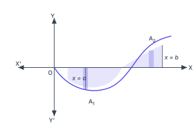
Fig 8.4 is the textbook’s key illustration for handling curves that cross the x-axis. It shows a single continuous curve $y = f(x)$ that behaves in two distinct parts between the vertical lines $x = a$ and $x = b$.

On the left, from $x = a$ up to some intermediate point, the curve dips below the x-axis, forming a lower lobe. This region is labelled $A_1$. Because every point on the curve here has a negative $y$-coordinate, the elementary strip of area $dA = y\,dx$ is negative. The integral $\int_a^{\text{crossing}} f(x)\,dx$ therefore gives a negative number for $A_1$.

After crossing the x-axis, the curve rises above it into an upper lobe on the right, labelled $A_2$. Here $y > 0$, so the elementary strips are positive, and $\int_{\text{crossing}}^b f(x)\,dx$ yields a positive value for $A_2$.

Both lobes are shaded indigo in the figure, but the shading carries a crucial message: area is a physical quantity that cannot be negative. The signed integral alone would cancel part of $A_1$ against $A_2$, giving a misleading result. The figure teaches that the actual bounded area is the sum of the absolute values:

where $c$ is the x-coordinate where the curve meets the axis (the point where $f(x)=0$). In the figure, $x=a$ and $x=b$ are the left and right boundaries, and the elementary strip at a general $x$ is drawn as a thin vertical rectangle of height $|y|$ and width $dx$.