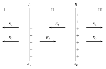
Q.Using theorem of superposition derive the expression for the electric field intensity due to a discrete charge distribution consisting of 'n' charges. If the charges are distributed continuously along a given length with charge density $\lambda$ then deduce the expression for the electric field in this case. (3+2=5) OR Two thin plane sheet of charge having charge density of $\sigma_1$ and $\sigma_2$ are placed parallel to each other. Derive the expression for the electric field intensities in the regions I, II and III as shown in figure. How will the intensity changed if the charge densities on the plates become $\sigma$ and $-\sigma$ respectively? (3+2=5)

Linear charge density lambda = charge / length, so its SI unit is coulomb per metre.

Linear charge density is defined as lambda = q/l, the charge distributed per unit length of a line/wire. Since charge is in …

For like charges the null point lies between them, nearer the smaller charge. Solving kq/x² = 4kq/(0·18−x)² gives x = 0·06 m from the smaller charge. Option (b).

Let the smaller charge be q and the larger 4q, separated by d = 0·18 m. The neutral point (E = 0) lies between them (both being of the same sign) at distance x from q.

Step 1 — equate field magnitudes:

kq/x² = k(4q)/(d−x)².

Step 2 — cancel kq and take square roots:

(d−x)²/x² = 4 → (d−x)/x = 2 → d − x = 2x → d = 3x.

…

Linear charge density is charge per unit length, so its unit is coulomb/metre.

Linear charge density is defined as the charge distributed per unit length of a line: $\lambda = \dfrac{q}{L}$.

…

The upper half of the ring (containing +q, near A) and the lower half (containing -q, near C) both produce a field at O pointing from A towards C -- so the resultant field at O genuinely is along OC. Assertion (A) is true. But equal and opposite charges at the same distance from O contribute equal and opposite potentials that exactly cancel, so the net potential at O is zero -- the opposite of what Reason (R) claims. Option (C).

Surface charge density σ = Q/A.

Surface density of charge is the charge distributed per unit area of a surface:

$\sigma = \frac{Q}{A}$

…

Surface charge density σ = charge/area.

Charge can be distributed along a line, over a surface, or through a volume, giving three densities. The surface (or superficial) charge density σ is defined as the charge per unit surface area:

$\sigma = \frac{q}{A}$

…

Surface charge density is charge per unit surface area, $\sigma = q/A$, measured in $\text{C/m}^2$.

When electric charge is distributed over a two-dimensional surface (such as the surface of a charged conductor or a charged plate), it is convenient to describe how densely the charge is packed using surface charge density.

It is defined as the charge $q$ present per unit area $A$ of the surface:

$\sigma = \frac{q}{A}$

…

The net force on a charge due to many other charges is just the vector sum of the pairwise Coulomb forces.

Coulomb's law gives the force between only two point charges. When more than two charges are present, the principle of superposition extends this to any number of charges.

It states that the force on any charge $q_0$ due to a group of charges $q_1, q_2, \dots, q_n$ is the vector sum of the forces exerted individually by each charge on $q_0$, each computed by Coulomb's law as if the other charges were not present:

$\vec{F} = \vec{F}_1 + \vec{F}_2 + \dots + \vec{F}_n = \sum_{i=1}^{n} \frac{1}{4\pi\epsilon_0}\frac{q_0 q_i}{r_i^2}\hat{r}_i$ …