Economics · Ch 4 — The Theory of the Firm under Perfect Competition

Short Run Supply Curve of a Firm

4.4.1

Short Run Supply Curve of a Firm

The Short Run Supply Curve of a Firm

The short run supply curve of a firm tells us how much output the firm will produce at each possible market price, given that its plant size is fixed. The derivation is done in two steps, depending on whether the market price is high enough to cover the firm’s variable costs.

Case 1: Market Price is Greater Than or Equal to the Minimum AVC

Suppose the market price is $p_1$ , and this price is above the minimum point of the Average Variable Cost (AVC) curve. The firm’s first step is to find the output level where price equals Short Run Marginal Cost (SMC). Because the SMC curve is U-shaped, there are two points where $p_1 = SMC$ — one on the falling part and one on the rising part. The profit-maximising firm chooses the output on the rising part of the SMC curve. Let this output be $q_1$ .

At $q_1$ , we must check the three conditions for profit maximisation in the short run:

Price equals SMC: $p_1 = SMC(q_1)$ .
SMC is rising at $q_1$ (we are on the upward-sloping segment).
Price is greater than or equal to AVC at $q_1$ : $p_1 \ge AVC(q_1)$ .

Since $p_1$ exceeds the minimum AVC, condition 3 is automatically satisfied at the chosen output $q_1$ . Therefore, when the market price is $p_1$ , the firm’s short run supply is exactly $q_1$ units.

Note

The condition $p \ge AVC$ is crucial. If price were below AVC, the firm would be making a loss on every unit produced — a loss larger than its fixed costs. In that case, shutting down (producing zero) is the better option.

Case 2: Market Price is Less Than the Minimum AVC

Now consider a market price $p_2$ that is lower than the minimum point of the AVC curve. For any positive output level, the AVC is strictly greater than $p_2$ . This means condition 3 — that price must be at least as large as AVC — can never be satisfied for any positive output.

If the firm produced any positive amount, its total variable cost would exceed its total revenue, and the loss would be greater than the fixed cost. The firm minimises its loss by producing zero output. In the short run, it still has to pay its fixed costs, but by producing nothing it avoids the additional variable costs that would only deepen the loss.

Watch out

A common mistake is to think the firm should produce if price is above AVC at some output. The correct rule is: the firm must check whether price is above AVC at the profit-maximising output (where $p = SMC$ ). If that output’s AVC is above price, the firm shuts down.

Combining the Two Cases: The Short Run Supply Curve

Putting the two cases together gives the complete short run supply curve of a perfectly competitive firm:

For any market price greater than or equal to the minimum AVC, the firm supplies the output level given by the rising part of the SMC curve.
For any market price strictly less than the minimum AVC, the firm supplies zero output.

In graphical terms, the short run supply curve is the rising portion of the SMC curve from the minimum point of the AVC curve upward, plus the vertical axis (representing zero output) for all prices below that minimum AVC.

Important

The short run supply curve is not the entire SMC curve. The downward-sloping part of SMC is irrelevant for supply decisions because a profit-maximising firm never chooses an output on that segment. Only the upward-sloping segment above the AVC minimum matters.

What the Textbook’s Figure Shows …

Figure 4.7Market Price Values. The figure shows the output levels chosen by a profit-maximising firm in the short run for two values of the market price: p₁ and p₂. When the market price is p₁, the output level of the firm is q₁; when the market price is p₂, the firm produces zero output.

Fig. 4.7 — Market Price Values. The figure shows the output levels chosen by a profit-maximising firm in the short run for two values of the market price: p₁ and p₂. When the market price is p₁, the output level of the firm is q₁; when the market price is p₂, the firm produces zero output.

Drawn by us to help you understand the concept clearly, and verified to make sure it's accurate. For exams, practice from your textbook's own diagram.

This figure is a short-run supply decision diagram for a perfectly competitive firm. It is not a market diagram — it shows only the firm’s cost curves and two horizontal price lines. The core lesson is that a profit-maximising firm does not always produce; below a certain price, it shuts down and produces zero.

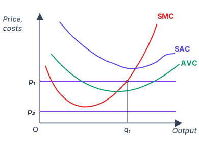
The vertical axis is labelled price/cost (in rupees per unit). The horizontal axis is labelled output (in units per period). Three curves are drawn: the short-run marginal cost (SMC) curve, U-shaped with a steeply rising right arm; the average variable cost (AVC) curve, which is U-shaped; and the short-run average cost (SAC) curve, also U-shaped and lying above the AVC curve. Two solid horizontal lines represent two different market prices: $p_1$ (higher) and $p_2$ (lower).

The physical idea is straightforward. A profit-maximising firm chooses output where price equals marginal cost, provided price is at least as high as the minimum of average variable cost. If price falls below that minimum, the firm cannot cover its variable costs and is better off producing nothing — it loses only its fixed costs, which are sunk in the short run.

When the market price is $p_1$ , the horizontal price line intersects the rising part of the SMC curve at a point above the AVC curve. The firm produces output $q_1$ , where $p_1 = SMC$ . In the figure as printed, $p_1$ still lies below the minimum of the SAC curve, so at $q_1$ the firm makes a loss — but because $p_1$ covers average variable cost, producing $q_1$ loses less than shutting down.

When the market price is $p_2$ , the price line lies below the minimum point of the AVC curve. The MC curve does intersect the price line at some output, but that output would not cover variable costs. The firm chooses $q = 0$ — it shuts down. The figure marks this by showing no output for $p_2$ .

Important

The shut-down point is the minimum of the AVC curve. Below that price, the firm produces zero in the short run. Above it, the firm produces along its MC curve.

The textbook uses this figure to derive the short-run supply curve of the firm. The key formula is the profit-maximisation condition:

P = MC(q)

where $P$ is the market price (taken as given by the firm) and $MC(q)$ is the marginal cost at output $q$ . This condition holds only for outputs where $P \ge \min AVC$ . The firm’s short-run supply curve is therefore the portion of the MC curve that lies above the minimum of the AVC curve.

q^*(P) = \begin{cases} \text{the } q \text{ such that } P = MC(q), & \text{if } P \ge \min AVC \\ 0, & \text{if } P < \min AVC \end{cases}

Here $q^*(P)$ is the profit-maximising output, $P$ is the market price, $MC(q)$ is marginal cost, and $\min AVC$ is the lowest value of average variable cost. The figure makes this piecewise rule visually clear: at $p_1$ the firm is on the MC curve; at $p_2$ it jumps to zero.

Watch out

Do not confuse the shut-down condition with the break-even condition. The break-even price is the minimum of ATC — above that, the firm earns positive profit. The shut-down price is the minimum of AVC — below that, the firm stops producing even if it could cover some fixed costs. …

Figure 4.8The Short Run Supply Curve of a Firm. The short run supply curve of a firm, which is based on its short run marginal cost curve (SMC) and average variable cost curve (AVC), is represented by the bold line.

Fig. 4.8 — The Short Run Supply Curve of a Firm. The short run supply curve of a firm, which is based on its short run marginal cost curve (SMC) and average variable cost curve (AVC), is represented by the bold line.

Drawn by us to help you understand the concept clearly, and verified to make sure it's accurate. For exams, practice from your textbook's own diagram.

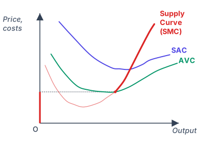
The figure plots three curves on a standard pair of axes. The vertical axis is labelled price/cost (in rupees), and the horizontal axis is labelled output (in units). Three curves are drawn: the short-run marginal cost curve (SMC), the short-run average cost curve (SAC) and the average variable cost curve (AVC). The SMC curve is U-shaped, first falling then rising. The SAC and AVC curves are also U-shaped, with SAC lying above AVC throughout. The SMC and AVC curves intersect at the minimum point of the AVC curve — that is, the SMC curve cuts the AVC curve from below at the AVC’s lowest point.

The short-run supply curve of the firm is shown as a bold line that follows a specific path. It begins at the point where the SMC curve meets the AVC curve (the minimum of AVC). From that point onward, the bold line traces the rising portion of the SMC curve that lies above the AVC curve. The portion of the SMC curve that lies below the AVC curve is not part of the supply curve. In other words, the firm’s short-run supply curve is the segment of the SMC curve that is above the AVC curve, starting at the shut-down point. For prices below the minimum AVC the firm supplies zero output, so the supply curve also includes a bold segment of the vertical (price) axis up to the minimum-AVC level, joined to the SMC segment by a dotted horizontal line in the figure.

Important

The short-run supply curve of a perfectly competitive firm is the rising part of its SMC curve that lies above the AVC curve. Below the minimum AVC, the firm supplies zero output.

The physical idea is this: in the short run, a firm must cover its variable costs to stay open. If the market price falls below the minimum average variable cost, the firm cannot even cover its variable costs — it is better to shut down and produce nothing. If the price is exactly at the minimum AVC, the firm is indifferent between producing and shutting down (the shut-down point). For any price above that minimum, the firm chooses the output level where price equals marginal cost (since $P = MR$ under perfect competition), and that output is read off the SMC curve. Because the SMC curve is rising in that region, a higher price leads to a higher quantity supplied — hence the supply curve slopes upward.

The key formula the textbook develops with this figure is the profit-maximising condition for a price-taking firm in the short run:

P = SMC(q)

where $P$ is the market price (which equals the firm’s marginal revenue $MR$ ), and $SMC(q)$ is the short-run marginal cost at output $q$ . The firm chooses $q$ such that this equality holds, provided $P \ge \min AVC$ . If $P < \min AVC$ , the firm produces $q = 0$ .

A second important relation is the shut-down condition: …

Start your 14-day free trial to unlock the full solution →

← Previous · 4.4Supply Curve of a Firm Next · 4.4.2 →Long Run Supply Curve of a Firm