Mathematics · Ch 5 — Linear Inequalities

Algebraic Solutions of Linear Inequalities in One Variable and Their Graphical Representation

5.3

Algebraic Solutions of Linear Inequalities in One Variable and Their Graphical Representation

Algebraic Solutions of Linear Inequalities in One Variable

When we solve an inequality, we are looking for all values of the variable that make the inequality true. These values are called the solutions of the inequality, and the collection of all such values is its solution set.

Consider the inequality $30x < 200$ . If $x$ represents the number of packets of rice, $x$ cannot be negative or a fraction. Testing values: $x = 0$ gives $0 < 200$ (true), $x = 1$ gives $30 < 200$ (true), and so on up to $x = 6$ giving $180 < 200$ (true). But $x = 7$ gives $210 < 200$ (false). So the solution set is $\{0, 1, 2, 3, 4, 5, 6\}$ .

This trial-and-error method is inefficient. We need systematic rules, just as we have for solving equations.

Rules for Solving Inequalities

When solving linear equations, we use two rules: adding the same number to both sides, and multiplying or dividing both sides by the same non-zero number. For inequalities, the rules are similar but with one critical difference.

Important

Rule 1: Equal numbers may be added to (or subtracted from) both sides of an inequality without affecting the sign of inequality.

Rule 2: Both sides of an inequality can be multiplied (or divided) by the same positive number. But when both sides are multiplied or divided by a negative number, the sign of inequality is reversed (i.e., $<$ becomes $>$ , $\leq$ becomes $\geq$ , and so on).

The reversal for negative numbers is not arbitrary. Consider $3 > 2$ . Multiply both sides by $-2$ : $3(-2) = -6$ and $2(-2) = -4$ . Since $-6 < -4$ , the inequality sign has reversed. Similarly, $-8 < -7$ but $(-8)(-2) > (-7)(-2)$ , i.e., $16 > 14$ .

Watch out

A common mistake is forgetting to reverse the inequality sign when multiplying or dividing by a negative number. Always check: if you multiply or divide by a negative, flip the sign.

Solving Step by Step

The method is straightforward: use Rule 1 to move terms, and Rule 2 to isolate the variable, being careful about sign reversal.

Example 1: Solve $30x < 200$ when

$x$ is a natural number,
$x$ is an integer. Divide both sides by 30 (positive, so no sign change): $\frac{30x}{30} < \frac{200}{30} \quad \Rightarrow \quad x < \frac{20}{3}$

(i) For natural numbers ( $1, 2, 3, \ldots$ ), the values satisfying $x < \frac{20}{3}$ are $1, 2, 3, 4, 5, 6$ . Solution set: $\{1, 2, 3, 4, 5, 6\}$ .

(ii) For integers ( $\ldots, -3, -2, -1, 0, 1, 2, \ldots$ ), the values satisfying $x < \frac{20}{3}$ are $\ldots, -3, -2, -1, 0, 1, 2, 3, 4, 5, 6$ . Solution set: $\{\ldots, -3, -2, -1, 0, 1, 2, 3, 4, 5, 6\}$ .

Example 2: Solve $5x - 3 < 3x + 1$ when

(i) $x$ is an integer,

(ii) $x$ is a real number.

Add 3 to both sides (Rule 1):

5x - 3 + 3 < 3x + 1 + 3 \quad \Rightarrow \quad 5x < 3x + 4

Subtract $3x$ from both sides (Rule 1):

5x - 3x < 3x + 4 - 3x \quad \Rightarrow \quad 2x < 4

Divide both sides by 2 (positive, no sign change):

x < 2

(i) For integers: $\ldots, -4, -3, -2, -1, 0, 1$ . Solution set: $\{\ldots, -4, -3, -2, -1, 0, 1\}$ .

(ii) For real numbers: all real numbers less than 2. Solution set: $x \in (-\infty, 2)$ .

Note

Unless stated otherwise, from now on we solve inequalities in the set of real numbers. The solution set is expressed using interval notation.

Example 3: Solve $4x + 3 < 6x + 7$ .

Subtract $6x$ from both sides:

4x - 6x + 3 < 6x + 7 - 6x \quad \Rightarrow \quad -2x + 3 < 7

Subtract 3 from both sides:

-2x < 4

Divide by $-2$ (negative — reverse the sign!):

x > -2

Solution set: $(-2, \infty)$ .

Example 4: Solve $\frac{5 - 2x}{3} \leq \frac{x}{6} - 5$ .

Multiply both sides by 6 (positive):

2(5 - 2x) \leq x - 30

10 - 4x \leq x - 30

Subtract $x$ from both sides:

10 - 5x \leq -30

Subtract 10 from both sides:

-5x \leq -40

Divide by $-5$ (negative — reverse the sign!):

x \geq 8

Solution set: $[8, \infty)$ .

Graphical Representation on the Number Line

The solution of an inequality in one variable can be shown on a number line.

Important

To represent $x < a$ (or $x > a$ ), put an open circle on the number $a$ and darken the line to the left (or right) of $a$ .
To represent $x \leq a$ (or $x \geq a$ ), put a closed (dark) circle on the number $a$ and darken the line to the left (or right) of $a$ .

Example 5: Solve $7x + 3 < 5x + 9$ and show the graph.

7x + 3 < 5x + 9

2x < 6

x < 3

On the number line, put an open circle at 3 and darken the line to the left.

Example 6: Solve $\frac{3x - 4}{2} \geq \frac{x + 1}{4} - 1$ and show the graph.

\frac{3x - 4}{2} \geq \frac{x + 1}{4} - 1

Multiply by 4:

2(3x - 4) \geq (x + 1) - 4

6x - 8 \geq x - 3

5x \geq 5

x \geq 1

On the number line, put a closed circle at 1 and darken the line to the right.

Applications: Word Problems

Inequalities model real-world constraints like minimum averages, ranges, and limits.

Example 7: A student scored 62 and 48 in two tests. Find the minimum marks needed in the third test to have an average of at least 60.

Let $x$ be the third test marks. The average condition:

\frac{62 + 48 + x}{3} \geq 60

110 + x \geq 180

x \geq 70

The student needs at least 70 marks.

Example 8: Find all pairs of consecutive odd natural numbers, both larger than 10, whose sum is less than 40.

Let the smaller odd number be $x$ . Then the next consecutive odd number is $x + 2$ .

Conditions:

x > 10 \quad \text{(1)}

x + (x + 2) < 40 \quad \text{(2)}

From (2): $2x + 2 < 40 \Rightarrow x < 19$ .

Combining: $10 < x < 19$ . Since $x$ is odd, $x$ can be 11, 13, 15, 17.

The pairs are: $(11, 13)$ , $(13, 15)$ , $(15, 17)$ , $(17, 19)$ .

Solving Systems of Inequalities (Compound Inequalities)

Sometimes we have two inequalities that must be satisfied simultaneously. We solve each separately and find the intersection of their solution sets.

Example 9: Solve $-8 \leq 5x - 3 < 7$ .

This is two inequalities: $-8 \leq 5x - 3$ and $5x - 3 < 7$ . Solve together:

-8 \leq 5x - 3 < 7

Add 3 to all three parts:

-5 \leq 5x < 10

Divide by 5:

-1 \leq x < 2

Solution set: $[-1, 2)$ .

Example 10: Solve $-5 \leq \frac{5 - 3x}{2} \leq 8$ .

Multiply all parts by 2:

-10 \leq 5 - 3x \leq 16

Subtract 5 from all parts:

-15 \leq -3x \leq 11

Divide by $-3$ (negative — reverse both inequalities):

5 \geq x \geq -\frac{11}{3}

This is written as $-\frac{11}{3} \leq x \leq 5$ .

Example 11: Solve the system:

3x - 7 < 5 + x \quad \text{(1)}

11 - 5x \leq 1 \quad \text{(2)}

From (1): $3x - x < 5 + 7 \Rightarrow 2x < 12 \Rightarrow x < 6$ . …

Figure 5.1Solution of 7x + 3 < 5x + 9 (i.e. x < 3) on the number line

Fig. 5.1 — Solution of 7x + 3 < 5x + 9 (i.e. x < 3) on the number line

Drawn by us to help you understand the concept clearly, and verified to make sure it's accurate. For exams, practice from your textbook's own diagram.

Fig. 5.1 is a simple but essential diagram: a horizontal number line with arrowheads on both ends, showing integer ticks around the number 3. A thick indigo ray starts at 3 and extends leftwards toward $-\infty$ , with an arrowhead at its left end. The point 3 itself is marked with an open (hollow) circle.

The open circle at 3 is the critical visual cue. It tells you that 3 is not included in the solution set — the inequality is strict ( $x < 3$ , not $x \leq 3$ ). The thick ray to the left represents all real numbers less than 3, stretching without bound in the negative direction. The arrowhead on the ray reinforces that the set continues indefinitely.

This figure teaches the standard method for graphing a one-variable linear inequality on the real number line. The inequality in question is $7x + 3 < 5x + 9$ , which simplifies to $x < 3$ . The diagram is the graphical counterpart of the algebraic solution: it shows every real number $x$ that makes the original statement true.

7x + 3 < 5x + 9 \quad \Longrightarrow \quad x < 3

The key idea is that a strict inequality ( $<$ or $>$ ) gets an open circle on the boundary point, while a non-strict inequality ( $\leq$ or $\geq$ ) would get a filled (closed) circle. The ray always points in the direction of the inequality sign: for $x < a$ , the ray goes left; for $x > a$ , it goes right.

Watch out

A common mistake is to draw a filled circle at 3 for $x < 3$ . Remember: open means the boundary is excluded; filled means it is included. Mixing these up will cost you marks in exams. …

Figure 5.2Solution x ≥ 1 on the number line

Fig. 5.2 — Solution x ≥ 1 on the number line

Drawn by us to help you understand the concept clearly, and verified to make sure it's accurate. For exams, practice from your textbook's own diagram.

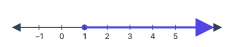
Fig. 5.2 is the graphical representation of the solution of the inequality solved in Example 6:

\frac{3x-4}{2} \geq \frac{x+1}{4} - 1

which simplifies to $x \geq 1$ .

The figure shows a horizontal number line with integer ticks marked around 1. The solution set $x \geq 1$ is drawn as a thick indigo ray that starts at the point corresponding to 1 and extends to the right (towards $+\infty$ ), ending in an arrowhead to indicate that it continues without bound. The point 1 itself is marked with a filled (solid) circle, because the inequality is inclusive — the value 1 is part of the solution set.

This is the standard way to represent an inequality of the form $x \geq a$ on a number line: a solid dot at $a$ and a thick ray to the right. If the inequality were strict ( $x > 1$ ), the circle would be open (unfilled), signalling that the endpoint is excluded.

Important

The solid circle at 1 means 1 is included in the solution set. For a strict inequality like $x > 1$ , you would use an open circle instead.

The key idea the figure teaches is that the solution set of a linear inequality in one variable is an interval (or a union of intervals) on the real number line, and the graphical representation makes it immediately clear which values satisfy the inequality.

The algebraic work that leads to this graph is:

\frac{3x-4}{2} \geq \frac{x+1}{4} - 1

Multiply through by 4 (a positive number, so the inequality direction stays the same):

2(3x-4) \geq (x+1) - 4

6x - 8 \geq x - 3

5x \geq 5

x \geq 1

So the solution set is all real numbers $x$ such that $x \geq 1$ , written in interval notation as $[1, \infty)$ . The square bracket at 1 indicates inclusion; the parenthesis at $\infty$ is always open because infinity is not a number you can reach. …

Figure 5.3Common solution of the system x < 6 and x ≥ 2 (i.e. 2 ≤ x < 6)

Fig. 5.3 — Common solution of the system x < 6 and x ≥ 2 (i.e. 2 ≤ x < 6)

Drawn by us to help you understand the concept clearly, and verified to make sure it's accurate. For exams, practice from your textbook's own diagram.

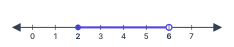
Fig. 5.3 is a simple but essential diagram: a horizontal number line with integer marks from 0 to 7. A thick segment runs from 2 to 6. At 2, the segment starts with a filled (solid) circle; at 6, it ends with an open (unfilled) circle. The thick segment itself is the common solution of the two inequalities $x < 6$ and $x \ge 2$ .

The filled circle at 2 means that 2 is included in the solution set — the inequality $x \ge 2$ allows equality. The open circle at 6 means that 6 is excluded — the inequality $x < 6$ does not allow equality. So the diagram shows every real number from 2 up to, but not including, 6. In interval notation, that is $[2, 6)$ .

The physical idea is straightforward: when you have two conditions that must hold simultaneously (a system of inequalities), the solution is the overlap of their individual solution sets. The number line makes that overlap visible at a glance. You read the diagram from left to right: start at the filled circle (included), move along the thick line, and stop just before the open circle (excluded).

Watch out

A common mistake is to confuse the open and filled circles. Remember: filled = included (the variable can equal that number), open = excluded (the variable cannot equal that number). If you reverse them, you get the wrong solution set.

The textbook develops this figure in Example 11, where the system is:

3x - 7 < 5 + x \quad \text{and} \quad 11 - 5x \le 1

Solving the first gives $x < 6$ ; solving the second gives $x \ge 2$ . The figure then shows the common solution $2 \le x < 6$ . …

Start your 14-day free trial to unlock the full solution →

← Previous · 5.2Inequalities Next · 5.3 →Example 1 — Solve 30x < 200 when (i) x is a natural number, (ii) x is an integer.