Mathematics · Ch 12 — Limits and Derivatives

Limits

12.3

Limits

The Idea of a Limit

The concept of a limit is the foundation of calculus. It answers a simple but powerful question: as the input to a function gets arbitrarily close to some number, what value does the output approach? This is not the same as asking what the function's value is at that point — the function might not even be defined there. The limit is about the trend of the function's values as we zoom in on a point.

Consider the function $f(x) = x^2$ . As $x$ takes values very close to $0$ , the value of $f(x)$ also moves towards $0$ . We write this as

\lim_{x \to 0} f(x) = 0

which is read as "the limit of $f(x)$ as $x$ tends to zero equals zero." The limit is the value $f(x)$ should assume at $x = 0$ , based on its behaviour near $0$ .

In general, if as $x \to a$ , $f(x) \to l$ , then $l$ is called the limit of the function $f(x)$ , written symbolically as

\lim_{x \to a} f(x) = l

Now take the function $g(x) = |x|$ , defined for $x \neq 0$ . Notice that $g(0)$ is not defined. But if we compute $g(x)$ for values of $x$ very close to $0$ , we see that the value of $g(x)$ moves towards $0$ . So

\lim_{x \to 0} g(x) = 0

This is intuitively clear from the graph of $y = |x|$ for $x \neq 0$ — the graph approaches the point $(0,0)$ from both sides, even though the point itself is missing.

Consider another function:

h(x) = \frac{x^2 - 4}{x - 2}, \quad x \neq 2

Compute $h(x)$ for values of $x$ very near to $2$ (but not at $2$ ). For $x = 1.9$ , $h(x) = 3.9$ ; for $x = 1.99$ , $h(x) = 3.99$ ; for $x = 2.01$ , $h(x) = 4.01$ . All these values are near $4$ . The graph of $y = h(x)$ confirms this — it is the line $y = x + 2$ with a hole at $x = 2$ , and as $x$ approaches $2$ , the $y$ -value approaches $4$ .

In all these examples, the value the function should assume at $x = a$ did not depend on how $x$ approaches $a$ . But there are essentially two ways $x$ can approach a number $a$ : from the left (values less than $a$ ) or from the right (values greater than $a$ ). This leads to two distinct concepts — the left-hand limit and the right-hand limit.

Left-Hand and Right-Hand Limits

Consider the function

f(x) = \begin{cases} 1, & x \leq 0 \\ 2, & x > 0 \end{cases}

The graph of this function is a horizontal line at $y = 1$ for $x \leq 0$ , and a horizontal line at $y = 2$ for $x > 0$ , with a jump at $x = 0$ .

The value of $f$ at $0$ dictated by values of $f(x)$ with $x \leq 0$ equals $1$ . This is the left-hand limit of $f(x)$ at $0$ :

\lim_{x \to 0^-} f(x) = 1

The value of $f$ at $0$ dictated by values of $f(x)$ with $x > 0$ equals $2$ . This is the right-hand limit of $f(x)$ at $0$ :

\lim_{x \to 0^+} f(x) = 2

Since the right and left-hand limits are different, we say that the limit of $f(x)$ as $x$ tends to zero does not exist — even though the function is defined at $0$ .

Important

The limit $\displaystyle \lim_{x \to a} f(x)$ exists if and only if both the left-hand limit and the right-hand limit exist and are equal. That common value is the limit.

Formal Definitions

We say $\displaystyle \lim_{x \to a^-} f(x)$ is the expected value of $f$ at $x = a$ given the values of $f$ near $x$ to the left of $a$ . This is the left-hand limit of $f$ at $a$ .

We say $\displaystyle \lim_{x \to a^+} f(x)$ is the expected value of $f$ at $x = a$ given the values of $f$ near $x$ to the right of $a$ . This is the right-hand limit of $f$ at $a$ .

If the right and left-hand limits coincide, we call that common value the limit of $f(x)$ at $x = a$ and denote it by $\displaystyle \lim_{x \to a} f(x)$ .

Illustrative Examples

Illustration 1: $f(x) = x + 10$ at $x = 5$

We compute the value of $f(x)$ for $x$ very near to $5$ .

$x$	4.9	4.95	4.99	4.995	5.001	5.01	5.1
$f(x)$	14.9	14.95	14.99	14.995	15.001	15.01	15.1

From the table, the value of $f(x)$ at $x = 5$ should be greater than $14.995$ and less than $15.001$ , assuming nothing dramatic happens between $x = 4.995$ and $x = 5.001$ . It is reasonable to assume that the value dictated by numbers to the left of $5$ is $15$ , i.e.,

\lim_{x \to 5^-} f(x) = 15

Similarly, when $x$ approaches $5$ from the right, $f(x)$ should take the value $15$ , i.e.,

\lim_{x \to 5^+} f(x) = 15

Hence the left and right-hand limits are both equal to $15$ , so

\lim_{x \to 5} f(x) = 15

The graph of $f(x) = x + 10$ is a straight line, and as $x$ approaches $5$ from either side, the graph approaches the point $(5, 15)$ . Notice that the value of the function at $x = 5$ also happens to be $15$ — the limit equals the function value.

Illustration 2: $f(x) = x^3$ at $x = 1$

$x$	0.9	0.99	0.999	1.001	1.01	1.1
$f(x)$	0.729	0.970299	0.997002999	1.003003001	1.030301	1.331

From the table, the value of $f(x)$ at $x = 1$ should be greater than $0.997002999$ and less than $1.003003001$ . The left-hand limit is $1$ , the right-hand limit is $1$ , so

\lim_{x \to 1} x^3 = 1

Again, the function value at $x = 1$ equals the limit.

Illustration 3: $f(x) = 3x$ at $x = 2$

$x$	1.9	1.95	1.99	1.999	2.001	2.01	2.1
$f(x)$	5.7	5.85	5.97	5.997	6.003	6.03	6.3

As $x$ approaches $2$ from either side, the value of $f(x)$ approaches $6$ . Hence

\lim_{x \to 2} 3x = 6

The function value at $x = 2$ coincides with the limit.

Illustration 4: Constant function $f(x) = 3$ at $x = 2$

A constant function takes the same value everywhere. Its value at points close to $2$ is $3$ . Hence

\lim_{x \to 2} 3 = 3

In fact, for any real number $a$ ,

\lim_{x \to a} 3 = 3

Illustration 5: $f(x) = x^2 + x$ at $x = 1$

$x$	0.9	0.99	0.999	1.01	1.1	1.2
$f(x)$	1.71	1.9701	1.997001	2.0301	2.31	2.64

It is reasonable to deduce that

\lim_{x \to 1} (x^2 + x) = 2

Again, $\lim_{x \to 1} f(x) = f(1) = 2$ .

Now, convince yourself of these three facts:

\lim_{x \to 1} x^2 = 1, \quad \lim_{x \to 1} x = 1, \quad \lim_{x \to 1} (x^2 + x) = 2

Then observe:

\lim_{x \to 1} (x^2 + x) = \lim_{x \to 1} x^2 + \lim_{x \to 1} x = 1 + 1 = 2

Also:

\lim_{x \to 1} [x(x+1)] = \left( \lim_{x \to 1} x \right) \cdot \left( \lim_{x \to 1} (x+1) \right) = 1 \cdot 2 = 2

This hints at the algebra of limits — limits can be added and multiplied.

Illustration 6: $f(x) = \sin x$ at $x = \frac{\pi}{2}$ (radians)

$x$	$\frac{\pi}{2} - 0.1$	$\frac{\pi}{2} - 0.01$	$\frac{\pi}{2} + 0.01$	$\frac{\pi}{2} + 0.1$
$f(x)$	0.9950	0.9999	0.9999	0.9950

From this, we deduce

\lim_{x \to \frac{\pi}{2}} \sin x = 1

The graph of $\sin x$ supports this. Here too, $\lim_{x \to \frac{\pi}{2}} \sin x = \sin \frac{\pi}{2} = 1$ .

Illustration 7: $f(x) = x + \cos x$ at $x = 0$

$x$	-0.1	-0.01	-0.001	0.001	0.01	0.1
$f(x)$	0.9850	0.98995	0.9989995	1.0009995	1.00995	1.0950

We deduce

\lim_{x \to 0} (x + \cos x) = 1

And indeed, $\lim_{x \to 0} f(x) = f(0) = 1$ .

Can you convince yourself that

\lim_{x \to 0} (x + \cos x) = \lim_{x \to 0} x + \lim_{x \to 0} \cos x

is true? This is the addition property of limits at work.

Illustration 8: $f(x) = \frac{1}{x^2}$ for $x > 0$ at $x = 0$

The domain of this function is all positive real numbers. It does not make sense to talk of $x$ approaching $0$ from the left. For positive $x$ close to $0$ :

$x$	1	0.1	0.01	$10^{-n}$
$f(x)$	1	100	10000	$10^{2n}$

As $x$ tends to $0$ , $f(x)$ becomes larger and larger — larger than any given number. Mathematically, we say

\lim_{x \to 0} f(x) = +\infty

Watch out

This is not a finite limit. The symbol $\infty$ does not represent a real number; it indicates that the function grows without bound. Such limits are not part of the standard Class 11 course.

Illustration 9: A piecewise function at $x = 0$

Consider

f(x) = \begin{cases} x - 2, & x < 0 \\ 0, & x = 0 \\ x + 2, & x > 0 \end{cases}

For negative $x$ , we use $x - 2$ ; for positive $x$ , we use $x + 2$ .

| $x$ | -0.1 | -0.01 | -0.001 | 0.001 | 0.01 | 0.1 |

|-----|------|-------|--------|-------|------|-----| …

Figure 12.2y = (x²−4)/(x−2): the line y = x+2 with a hole at (2, 4)

Fig. 12.2 — y = (x²−4)/(x−2): the line y = x+2 with a hole at (2, 4)

Drawn by us to help you understand the concept clearly, and verified to make sure it's accurate. For exams, practice from your textbook's own diagram.

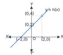
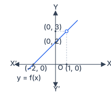
Fig. 12.2 is the graph of the function $h(x) = \frac{x^2 - 4}{x - 2}$ , defined for all $x \neq 2$ . The axes are the standard four-quadrant Cartesian axes. The curve drawn is the straight line $y = x + 2$ , which passes through $(-2,0)$ and $(0,2)$ .

The critical feature is an open circle (a hole) at the point $(2,4)$ . Dashed guide lines drop vertically from the hole to the $x$ -axis at $x=2$ and horizontally to the $y$ -axis at $y=4$ , making it clear that the function never actually reaches $(2,4)$ — the point is missing from the graph. The function is labelled $y = h(x)$ .

Watch out

The hole is not a break in the line — it is a single missing point. The line $y = x+2$ is continuous everywhere except at $x=2$ , where the original expression $\frac{x^2-4}{x-2}$ is undefined because division by zero is not allowed.

What this figure teaches. The central idea is that a function can approach a particular value as $x$ gets arbitrarily close to a point, even if the function is not defined at that point. As $x$ approaches $2$ from either side (left or right), the values of $h(x)$ get closer and closer to $4$ . The graph shows this visually: the line $y = x+2$ passes smoothly through every $x$ near $2$ , but the point $(2,4)$ is absent. The limit of $h(x)$ as $x \to 2$ is $4$ , even though $h(2)$ does not exist.

\lim_{x \to 2} \frac{x^2 - 4}{x - 2} = 4

Why the formula works. Factor the numerator: $x^2 - 4 = (x-2)(x+2)$ . For $x \neq 2$ , the factor $(x-2)$ cancels, leaving $h(x) = x+2$ . So the function is identical to the line $y = x+2$ everywhere except at $x=2$ . The limit is simply the value that line would have at $x=2$ , which is $2+2 = 4$ . The hole in the graph is the visual signature of a removable discontinuity — the function can be "repaired" by defining $h(2)=4$ , but the original definition leaves it missing. …

Figure 12.3Step function f(x)=1 (x≤0), 2 (x>0): left limit 1, right limit 2

Fig. 12.3 — Step function f(x)=1 (x≤0), 2 (x>0): left limit 1, right limit 2

Drawn by us to help you understand the concept clearly, and verified to make sure it's accurate. For exams, practice from your textbook's own diagram.

What Fig. 12.3 Shows

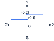
The figure plots a piecewise constant function defined as:

f(x) = \begin{cases} 1, & x \leq 0 \\ 2, & x > 0 \end{cases}

The axes are the standard four-quadrant Cartesian plane. On the left side of the vertical axis (for $x \leq 0$ ), you see a horizontal blue ray at height $y = 1$ . This ray ends exactly at the origin with a filled dot at $(0,1)$ — the filled dot tells you the function actually takes the value $1$ at $x = 0$ . On the right side of the vertical axis (for $x > 0$ ), there is a separate horizontal blue ray at height $y = 2$ . This ray begins at the origin with an open circle at $(0,2)$ — the open circle tells you the function does not take the value $2$ at $x = 0$ ; it only takes that value for $x$ strictly greater than $0$ .

The graph therefore has a jump at $x = 0$ : the left part sits at $y = 1$ , the right part sits at $y = 2$ , and there is a gap between the filled dot and the open circle.

The Physical Idea

This figure is the textbook's central example for understanding one-sided limits and why a limit may not exist even when the function is defined at the point. The key observation is that the behaviour of $f(x)$ as $x$ approaches $0$ depends entirely on which side you approach from.

If you approach $x = 0$ from the left (using values like $x = -0.1, -0.01, -0.001$ ), the function's value is always $1$ . The left-hand limit is therefore $1$ :

\lim_{x \to 0^-} f(x) = 1

If you approach $x = 0$ from the right (using values like $x = 0.001, 0.01, 0.1$ ), the function's value is always $2$ . The right-hand limit is therefore $2$ :

\lim_{x \to 0^+} f(x) = 2

Since these two one-sided limits are different numbers ( $1 \neq 2$ ), there is no single value that $f(x)$ "settles down to" as $x$ gets arbitrarily close to $0$ from both sides. Hence the two-sided limit does not exist:

\lim_{x \to 0} f(x) \text{ does not exist}

Watch out

A common mistake is to think that because the function is defined at $x = 0$ (it is — $f(0) = 1$ ), the limit must also exist. This figure shows the opposite: the function's value at the point and the limit as you approach that point are independent ideas. Here the function is defined, but the limit does not exist because the left and right behaviours disagree.

The Key Formula the Figure Develops

The textbook uses this figure to establish the formal definition of one-sided limits and the condition for the existence of a two-sided limit:

\lim_{x \to a} f(x) = L \quad \text{if and only if} \quad \lim_{x \to a^-} f(x) = \lim_{x \to a^+} f(x) = L

Figure 12.4f(x)=3x: sample points climb toward (2, 6) as x→2

Fig. 12.4 — f(x)=3x: sample points climb toward (2, 6) as x→2

Drawn by us to help you understand the concept clearly, and verified to make sure it's accurate. For exams, practice from your textbook's own diagram.

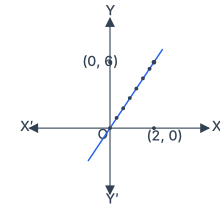
Fig. 12.4 is the graph of $f(x)=3x$ , drawn to illustrate what happens to the function’s value as $x$ gets closer and closer to $2$ . The axes are the standard four-quadrant Cartesian axes. The blue line is the straight line $y=3x$ , passing through the origin $(0,0)$ with slope $3$ . Along this line, a row of filled dots marches toward the point $(2,6)$ — these dots represent the function values at sample points like $x=1.9, 1.95, 1.99, 1.999$ on the left and $x=2.001, 2.01, 2.1$ on the right. The point $(2,6)$ itself is the target: as $x$ approaches $2$ from either side, the corresponding $y$ -values approach $6$ .

The figure also marks $(0,6)$ on the $y$ -axis and $(2,0)$ on the $x$ -axis. These are not points on the graph; they are reference markers that help you see the horizontal and vertical distances involved. The vertical line from $(2,0)$ up to $(2,6)$ and the horizontal line from $(0,6)$ across to $(2,6)$ frame the approach.

The physical idea is the core of the limit concept: the function $f(x)=3x$ is defined at $x=2$ (its value is $6$ ), but the limit asks what value the function tends toward as $x$ gets arbitrarily close to $2$ — not necessarily what it equals at $2$ . Here, the left-hand values (like $5.7, 5.85, 5.97, 5.997$ ) and the right-hand values (like $6.003, 6.03, 6.3$ ) both close in on $6$ . Because the left and right limits agree, the two-sided limit exists and equals $6$ .

The textbook uses this figure to introduce the notation and the equality of one-sided limits:

\lim_{x \to 2^-} f(x) = \lim_{x \to 2^+} f(x) = \lim_{x \to 2} f(x) = 6

Figure 12.5Graph of f(x) = x squared plus x illustrating that the function approaches the value 2 as x tends to 1, with dashed guide lines drawn to the point (1, 2).

Fig. 12.5 — Graph of f(x) = x squared plus x illustrating that the function approaches the value 2 as x tends to 1, with dashed guide lines drawn to the point (1, 2).

Drawn by us to help you understand the concept clearly, and verified to make sure it's accurate. For exams, practice from your textbook's own diagram.

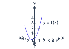
Fig. 12.5 is the graph of $f(x) = x^{2} + x$ , drawn to illustrate what it means for a function to approach a particular value as $x$ gets close to a point. The axes are marked with $x$ from $-2$ to $5$ and $y$ from $1$ to $4$ . The curve itself is an upward-opening parabola (indigo in the textbook) that passes through $(-1,0)$ and the origin, with its vertex near $(-0.5, -0.25)$ . The key feature is the point $(1,2)$ on the curve, from which a dashed horizontal guide line runs leftwards to the $y$ -axis. That guide is the visual clue: as $x$ moves toward $1$ from either side, the corresponding $y$ -values on the curve slide toward $2$ .

The physical idea is simple but foundational. You are not yet asking what $f(1)$ equals (though here it happens to be $2$ as well). Instead, you are watching the behaviour of the function in a neighbourhood of $x=1$ . The dashed line to the $y$ -axis shows that the $y$ -coordinate the curve is "aiming at" is $2$ . This is the limit: the number the outputs get arbitrarily close to as the inputs get arbitrarily close to $1$ , regardless of whether the function is actually defined at $1$ or not.

The textbook uses this figure to develop the limit statement for $f(x) = x^{2} + x$ at $x=1$ :

\lim_{x \to 1} (x^{2} + x) = 2

Here $\lim_{x \to 1}$ means "the limit as $x$ approaches $1$ ", and the expression inside the limit is the function $f(x) = x^{2} + x$ . The result $2$ is the common value of the left-hand limit and the right-hand limit — the $y$ -value the graph converges to from both directions. The figure makes this convergence visible: the curve smoothly meets the point $(1,2)$ , and the dashed guide emphasises that the $y$ -coordinate of that meeting point is $2$ .

The textbook then uses this concrete example to illustrate a general algebraic property: the limit of a sum is the sum of the limits. From the same figure and the table of values (Table 12.7), they show that

\lim_{x \to 1} (x^{2} + x) = \lim_{x \to 1} x^{2} + \lim_{x \to 1} x = 1 + 1 = 2

and also that

$\lim_{x \to 1} (x^{2} + x) = \left( \lim_{x \to 1} x \right) \left( \lim_{x \to 1} x \right) + \lim_{x \to 1} x = 1 \cdot 1 + 1 = 2.$ …

Figure 12.6f(x)=x−2 (x<0), 0 (x=0), x+2 (x>0): left limit −2, right limit 2, value 0

Fig. 12.6 — f(x)=x−2 (x<0), 0 (x=0), x+2 (x>0): left limit −2, right limit 2, value 0

Drawn by us to help you understand the concept clearly, and verified to make sure it's accurate. For exams, practice from your textbook's own diagram.

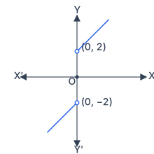
Fig 12.6 is the graph of a piecewise function that makes the idea of left-hand and right-hand limits visually concrete. The function is defined in three pieces:

f(x) = \begin{cases} x - 2, & x < 0 \\[4pt] 0, & x = 0 \\[4pt] x + 2, & x > 0 \end{cases}

The axes are the standard four-quadrant Cartesian plane. On the left side of the $y$ -axis (for $x < 0$ ), you see a blue straight line segment that follows $y = x - 2$ . This line rises as it moves rightward, but it stops just before reaching $x = 0$ — the endpoint at $(0, -2)$ is marked with an open circle, meaning the function does not take that value at $x = 0$ . On the right side of the $y$ -axis (for $x > 0$ ), a blue straight line segment follows $y = x + 2$ . This line also rises as it moves rightward, and it begins just after $x = 0$ with an open circle at $(0, 2)$ . At the origin itself, there is a filled dot at $(0, 0)$ , which is the actual value of the function at $x = 0$ .

The physical idea is this: as $x$ approaches $0$ from the left (through negative numbers), the $y$ -values of the function get closer and closer to $-2$ . That is the left-hand limit, written

\lim_{x \to 0^{-}} f(x) = -2.

As $x$ approaches $0$ from the right (through positive numbers), the $y$ -values get closer and closer to $2$ . That is the right-hand limit,

\lim_{x \to 0^{+}} f(x) = 2.

The two limits are different. Therefore, the two-sided limit $\displaystyle \lim_{x \to 0} f(x)$ does not exist — even though the function itself is defined at $x = 0$ and equals $0$ . The graph makes this crystal clear: the two arms of the function point toward different $y$ -values, so there is no single number that the function "wants" to approach at $x = 0$ .

Watch out

A common mistake is to think that if $f(0)$ exists, then the limit must also exist. This figure is the classic counterexample: the function has a value at $0$ , but the left and right limits disagree, so the limit does not exist.

The key formula the textbook develops with this figure is the definition of the existence of a limit: …

Figure 12.7f(x)=x+2 for x≠1 with f(1)=0: line y=x+2 with a hole at (1, 3)

Fig. 12.7 — f(x)=x+2 for x≠1 with f(1)=0: line y=x+2 with a hole at (1, 3)

Drawn by us to help you understand the concept clearly, and verified to make sure it's accurate. For exams, practice from your textbook's own diagram.

What Fig. 12.7 Shows

The figure plots the function

f(x) = \begin{cases} x+2, & x \neq 1 \\[4pt] 0, & x = 1 \end{cases}

on a standard four-quadrant coordinate system. The axes are drawn with the origin at the centre. A straight blue line represents $y = x+2$ across the entire plane. This line passes through $(-2,0)$ and $(0,2)$ , and continues in both directions with slope $1$ and $y$ -intercept $2$ .

The critical feature is at $x = 1$ . On the line $y = x+2$ , the point $(1,3)$ would normally lie. But the figure marks this location with an open circle — a hollow dot — indicating that the function is not defined there by the rule $x+2$ . Instead, the function value at $x=1$ is given separately as $f(1) = 0$ , which would be plotted at $(1,0)$ on the graph. Two dashed guide lines are drawn: one horizontal from the open circle at $(1,3)$ across to the $y$ -axis at $y=3$ , and one vertical from the same open circle down to the $x$ -axis at $x=1$ . These guides help the eye see the $y$ -coordinate that the function would have if it followed the line, versus the actual value at $x=1$ .

The graph is labelled $y = f(x)$ .

The Physical Idea

This figure teaches the central distinction between the limit of a function at a point and the value of the function at that point. As $x$ approaches $1$ from either side — whether through values like $0.9, 0.99, 0.999$ from the left, or $1.1, 1.01, 1.001$ from the right — the corresponding $f(x)$ values get arbitrarily close to $3$ . The open circle at $(1,3)$ captures this behaviour: the function wants to be $3$ at $x=1$ , even though it is actually defined to be $0$ there.

The dashed guide lines reinforce the idea visually. The horizontal guide shows the $y$ -value ( $3$ ) that the function approaches as $x$ nears $1$ . The vertical guide shows the $x$ -value ( $1$ ) at which this approach happens. Together, they frame the limit as the "expected" or "intended" value of the function at that $x$ , based on the behaviour of nearby points.

Watch out

A common mistake is to think the limit equals the function value. Fig. 12.7 explicitly shows they can be different: $\lim_{x \to 1} f(x) = 3$ , but $f(1) = 0$ . The limit is about approach, not arrival.

The Key Formula

The textbook uses this figure to illustrate the definition of a limit when the left-hand and right-hand limits coincide. For this function:

\lim_{x \to 1^-} f(x) = 3 \quad \text{and} \quad \lim_{x \to 1^+} f(x) = 3

Since both one-sided limits are equal, the two-sided limit exists:

\lim_{x \to 1} f(x) = 3

Table 12.4Values of $f(x) = x + 10$ as $x$ approaches 5

| $x$ | 4.9 | 4.95 | 4.99 | 4.995 | 5.001 | 5.01 | 5.1 |

|---|---|---|---|---|---|---|---| …

Table 12.5Values of $f(x) = x^3$ as $x$ approaches 1

| $x$ | 0.9 | 0.99 | 0.999 | 1.001 | 1.01 | 1.1 |

|---|---|---|---|---|---|---| …

Table 12.6Values of $f(x) = 3x$ as $x$ approaches 2

| $x$ | 1.9 | 1.95 | 1.99 | 1.999 | 2.001 | 2.01 | 2.1 |

|---|---|---|---|---|---|---|---| …

Table 12.7Values of $f(x) = x^2 + x$ as $x$ approaches 1

| $x$ | 0.9 | 0.99 | 0.999 | 1.01 | 1.1 | 1.2 |

|---|---|---|---|---|---|---| …

Table 12.8Values of $f(x) = \sin x$ as $x$ approaches $\frac{\pi}{2}$

| $x$ | $\frac{\pi}{2} - 0.1$ | $\frac{\pi}{2} - 0.01$ | $\frac{\pi}{2} + 0.01$ | $\frac{\pi}{2} + 0.1$ |

|---|---|---|---|---| …

Table 12.9Values of $f(x) = x + \cos x$ as $x$ approaches 0

| $x$ | $-0.1$ | $-0.01$ | $-0.001$ | 0.001 | 0.01 | 0.1 |

|---|---|---|---|---|---|---| …

Table 12.10Values of $f(x) = \frac{1}{x^2}$ for positive $x$ close to 0 ($n$ any positive integer)

| $x$ | 1 | 0.1 | 0.01 | $10^{-n}$ |

|---|---|---|---|---| …

Table 12.11Values of the piecewise function ($x-2$ for $x<0$, $0$ at $x=0$, $x+2$ for $x>0$) near 0

| $x$ | $-0.1$ | $-0.01$ | $-0.001$ | 0.001 | 0.01 | 0.1 |

|---|---|---|---|---|---|---| …

Table 12.12Values of the piecewise function ($x+2$ for $x \neq 1$, $0$ at $x=1$) near 1

| $x$ | 0.9 | 0.99 | 0.999 | 1.001 | 1.01 | 1.1 |

|---|---|---|---|---|---|---| …

Start your 14-day free trial to unlock the full solution →

← Previous · 12.2Intuitive Idea of Derivatives Next · 12.3.1 →Algebra of Limits

Limits

Limits

The Idea of a Limit

Left-Hand and Right-Hand Limits

Formal Definitions

Illustrative Examples

Illustration 1: f(x)=x+10f(x) = x + 10f(x)=x+10 at x=5x = 5x=5

Illustration 2: f(x)=x3f(x) = x^3f(x)=x3 at x=1x = 1x=1

Illustration 3: f(x)=3xf(x) = 3xf(x)=3x at x=2x = 2x=2

Illustration 4: Constant function f(x)=3f(x) = 3f(x)=3 at x=2x = 2x=2

Illustration 5: f(x)=x2+xf(x) = x^2 + xf(x)=x2+x at x=1x = 1x=1

Illustration 6: f(x)=sin⁡xf(x) = \sin xf(x)=sinx at x=π2x = \frac{\pi}{2}x=2π​ (radians)

Illustration 7: f(x)=x+cos⁡xf(x) = x + \cos xf(x)=x+cosx at x=0x = 0x=0

Illustration 8: f(x)=1x2f(x) = \frac{1}{x^2}f(x)=x21​ for x>0x > 0x>0 at x=0x = 0x=0

Illustration 9: A piecewise function at x=0x = 0x=0

What Fig. 12.3 Shows

The Physical Idea

The Key Formula the Figure Develops

What Fig. 12.7 Shows

The Physical Idea

The Key Formula

Illustration 1: $f(x) = x + 10$ at $x = 5$

Illustration 2: $f(x) = x^3$ at $x = 1$

Illustration 3: $f(x) = 3x$ at $x = 2$

Illustration 4: Constant function $f(x) = 3$ at $x = 2$

Illustration 5: $f(x) = x^2 + x$ at $x = 1$

Illustration 6: $f(x) = \sin x$ at $x = \frac{\pi}{2}$ (radians)

Illustration 7: $f(x) = x + \cos x$ at $x = 0$

Illustration 8: $f(x) = \frac{1}{x^2}$ for $x > 0$ at $x = 0$

Illustration 9: A piecewise function at $x = 0$