Physics · Ch 2 — Motion in a Straight Line

Instantaneous Velocity and Speed

2.2

Instantaneous Velocity and Speed

From Average to Instantaneous: The Core Idea

Average velocity tells you the overall rate of displacement over a finite time interval. But motion is rarely uniform — a car speeds up, slows down, stops at a light. The speedometer shows the velocity at this very instant, not an average over the last hour. That reading is the instantaneous velocity.

To capture this idea mathematically, we shrink the time interval $\Delta t$ to be extremely small — so small that over that interval the motion is essentially uniform. The average velocity over that tiny interval becomes a very good approximation of the velocity at the starting instant. As $\Delta t$ approaches zero, this approximation becomes exact.

Defining Instantaneous Velocity

Consider a particle moving along a straight line. Let its position at time $t$ be $x(t)$ . Choose a small time interval $\Delta t$ starting at $t$ . The displacement over this interval is $\Delta x = x(t + \Delta t) - x(t)$ , and the average velocity is

v_{\text{avg}} = \frac{\Delta x}{\Delta t}.

Now let $\Delta t$ become smaller and smaller — we take the limit $\Delta t \to 0$ . The value that the average velocity approaches is the instantaneous velocity at time $t$ :

v(t) = \lim_{\Delta t \to 0} \frac{\Delta x}{\Delta t}.

This limit is precisely the derivative of position with respect to time:

v(t) = \frac{dx}{dt}.

Important

Instantaneous velocity is the derivative of position with respect to time. It tells you both how fast and in which direction the particle is moving at a single instant.

The magnitude of instantaneous velocity is called instantaneous speed. Speed is always a non-negative quantity — it has no direction information.

Geometric Interpretation: The Slope of the Tangent

On a position–time ( $x$ – $t$ ) graph, the average velocity over an interval $\Delta t$ is the slope of the secant line joining the two points $(t, x(t))$ and $(t+\Delta t, x(t+\Delta t))$ .

As $\Delta t$ shrinks, the secant line rotates and approaches a line that just touches the curve at the single point $(t, x(t))$ — the tangent line. The slope of this tangent line is exactly $\frac{dx}{dt}$ , the instantaneous velocity.

Note

If the $x$ – $t$ graph is a straight line, the tangent line is the line itself — instantaneous velocity is constant and equals the average velocity over any interval.

Numerical Verification: Table 2.1

The limiting process described above can be checked numerically, not just graphically. For the curve $x = 0.08\,t^{3}$ shown in Fig. 2.1, Table 2.1 tabulates the value of $\Delta x/\Delta t$ for successively smaller intervals $\Delta t$ , each centred at $t = 4$ s, using $t_1 = \left(t - \dfrac{\Delta t}{2}\right)$ and $t_2 = \left(t + \dfrac{\Delta t}{2}\right)$ .

Table 2.1 Limiting value of $\dfrac{\Delta x}{\Delta t}$ at $t = 4$ s

$\Delta t$ (s)	$t_1$ (s)	$t_2$ (s)	$x(t_1)$ (m)	$x(t_2)$ (m)	$\Delta x$ (m)	$\Delta x/\Delta t$ (m s $^{-1}$ )
2.0	3.0	5.0	2.16	10.0	7.84	3.92
1.0	3.5	4.5	3.43	7.29	3.86	3.86
0.5	3.75	4.25	4.21875	6.14125	1.9225	3.845
0.1	3.95	4.05	4.93039	5.31441	0.38402	3.8402
0.01	3.995	4.005	5.100824	5.139224	0.0384	3.8400

As $\Delta t$ shrinks from 2.0 s down to 0.01 s, the value of $\Delta x/\Delta t$ steadily converges to $3.84$ m/s. This is exactly the instantaneous velocity at $t = 4$ s (point P) -- the same value the slope of the tangent line gives graphically in Fig. 2.1.

Properties of Instantaneous Velocity

The textbook lists three key properties that follow directly from the definition. Each is proved below.

›Proof

Property (I): If $x$ is a linear function of $t$ , instantaneous velocity is constant and equals the average velocity.

Let $x(t) = a + bt$ , where $a$ and $b$ are constants. Then

$v(t) = \frac{dx}{dt} = b.$

The average velocity over any interval $[t_1, t_2]$ is

$v_{\text{avg}} = \frac{x(t_2) - x(t_1)}{t_2 - t_1} = \frac{(a+bt_2) - (a+bt_1)}{t_2 - t_1} = \frac{b(t_2 - t_1)}{t_2 - t_1} = b.$

So $v(t) = v_{\text{avg}} = b$ for all $t$ .

›Proof

Property (II): Instantaneous velocity at a given time can be positive, negative, or zero.

From $v(t) = dx/dt$ :

If $x$ is increasing with $t$ , the slope of the tangent is positive → $v(t) > 0$ (motion in the positive direction).
If $x$ is decreasing with $t$ , the slope is negative → $v(t) < 0$ (motion in the negative direction).
If $x$ is momentarily constant (a turning point or a pause), the tangent is horizontal → $v(t) = 0$ .

›Proof

Property (III): For uniform motion (constant velocity), instantaneous velocity equals the constant average velocity at every instant.

Uniform motion means $x(t) = x_0 + vt$ , where $v$ is constant. Then

$v(t) = \frac{dx}{dt} = v.$

The average velocity over any interval is also $v$ , as shown in Property (I). So the two are identical.

Instantaneous Speed

Instantaneous speed is defined as the magnitude of instantaneous velocity: …

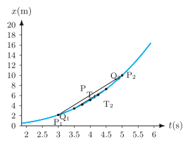
Figure 2.1Determining velocity from position-time graph. Velocity at t = 4 s is the slope of the tangent to the graph at that instant.

Fig. 2.1 — Determining velocity from position-time graph. Velocity at t = 4 s is the slope of the tangent to the graph at that instant.

Drawn by us to help you understand the concept clearly, and verified to make sure it's accurate. For exams, practice from your textbook's own diagram.

The figure plots position $x$ (in metres) on the vertical axis against time $t$ (in seconds) on the horizontal axis. The curve shown is $x = 0.08\,t^{3}$ , which rises steeply from $t = 2$ s to $t = 6$ s. On this curve, five points are marked: $P_{1}$ , $Q_{1}$ , $P$ , $Q_{2}$ , and $P_{2}$ , in that order from left to right. The central point $P$ corresponds to $t = 4$ s, the instant at which we want the velocity. Two chords are drawn: $P_{1}P_{2}$ (connecting a point before $P$ to a point after $P$ ) and $Q_{1}Q_{2}$ (connecting points closer to $P$ ). A tangent line is also drawn at $P$ , with its two ends labelled $T_{1}$ and $T_{2}$ .

The physical idea is that the average velocity over an interval equals the slope of the chord joining the two corresponding points on the $x$ - $t$ graph. As the interval shrinks — moving from chord $P_{1}P_{2}$ to the tighter chord $Q_{1}Q_{2}$ — the chord’s slope approaches the slope of the tangent at $P$ . In the limit where the time interval goes to zero, the average velocity becomes the instantaneous velocity, which is exactly the slope of the tangent line at that instant.

The key formula developed from this figure is the definition of instantaneous velocity:

v(t) = \lim_{\Delta t \to 0} \frac{x(t+\Delta t) - x(t)}{\Delta t} = \frac{dx}{dt}

Here $v(t)$ is the instantaneous velocity at time $t$ , $x(t)$ is the position at that time, $\Delta t$ is a small time interval, and $\frac{dx}{dt}$ is the derivative of position with respect to time — the slope of the tangent to the $x$ - $t$ graph at the point $(t, x(t))$ .

For the specific curve $x = 0.08\,t^{3}$ , the instantaneous velocity at $t = 4$ s is found by differentiating:

v(t) = \frac{d}{dt}(0.08\,t^{3}) = 0.24\,t^{2}

so at $t = 4$ s, $v = 0.24 \times 16 = 3.84$ m/s. This is the numerical value of the tangent’s slope shown in the figure. …

Start your 14-day free trial to unlock the full solution →

← Previous · 2.1Introduction Next · 2.2 →Example 2.1 — The position of an object moving along x-axis is given by x = a + bt² …