Mathematics · Ch 6 — Application of Derivatives

Increasing and Decreasing Functions

6.3

Increasing and Decreasing Functions

6.3 Increasing and Decreasing Functions

The Intuitive Idea

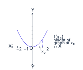
Consider $f(x) = x^2$ , a parabola opening upward. To the right of the origin ( $x > 0$ ), as we move left to right the height rises — the function is increasing. To the left ( $x < 0$ ), the height falls as we move left to right — the function is decreasing. We now make these observations precise.

Analytical Definitions on an Interval

Let $I$ be an interval contained in the domain of a real-valued function $f$ .

Definition 1: Types of Monotonic Behaviour on an Interval

(i) Increasing on $I$ : for all $x_1, x_2 \in I$ , $\;x_1 < x_2 \implies f(x_1) \leq f(x_2)$ (never goes down; may stay flat or go up).

(ii) Decreasing on $I$ : for all $x_1, x_2 \in I$ , $\;x_1 < x_2 \implies f(x_1) \geq f(x_2)$ (never goes up).

(iii) Constant on $I$ : $f(x) = c$ for all $x \in I$ , where $c$ is a constant.

(iv) Strictly increasing on $I$ : $x_1 < x_2 \implies f(x_1) < f(x_2)$ (always goes up, never flat).

(v) Strictly decreasing on $I$ : $x_1 < x_2 \implies f(x_1) > f(x_2)$ (always goes down).

Important

The difference between "increasing" and "strictly increasing" is the difference between $\leq$ and $<$ . A constant function is increasing but not strictly increasing.

Definition 2: Increasing/Decreasing at a Point

Let $x_0$ be in the domain of $f$ . Then $f$ is increasing at $x_0$ if there is an open interval $I$ containing $x_0$ on which $f$ is increasing, and decreasing at $x_0$ if there is such an interval on which $f$ is decreasing. This localises the concept to a small neighbourhood of a single point.

The First Derivative Test for Increasing/Decreasing Functions

Theorem 1

Let $f$ be continuous on $[a, b]$ and differentiable on $(a, b)$ . Then:

(a) $f$ is increasing in $[a, b]$ if $f'(x) > 0$ for each $x \in (a, b)$

(b) $f$ is decreasing in $[a, b]$ if $f'(x) < 0$ for each $x \in (a, b)$

(c) $f$ is a constant function in $[a, b]$ if $f'(x) = 0$ for each $x \in (a, b)$

›Proof

Part (a): Let $x_1, x_2 \in [a, b]$ with $x_1 < x_2$ . Since $f$ is continuous on $[x_1, x_2]$ and differentiable on $(x_1, x_2)$ , the Mean Value Theorem (Theorem 8 of Chapter 5) gives a point $c$ between them with

$f(x_2) - f(x_1) = f'(c)(x_2 - x_1).$

Given $f'(c) > 0$ and $x_2 - x_1 > 0$ , we get $f(x_2) - f(x_1) > 0$ , i.e. $f(x_1) < f(x_2)$ . So $f$ is increasing on $[a, b]$ .

Part (b): With $f'(c) < 0$ and $x_2 - x_1 > 0$ , $f(x_2) - f(x_1) < 0$ , so $f$ is decreasing.

Part (c): With $f'(c) = 0$ , $f(x_2) = f(x_1)$ , so $f$ is constant.

Note

A more general version: if $f'(x) > 0$ (resp. $< 0$ ) on the interior of an interval and $f$ is continuous there, then $f$ is increasing (resp. decreasing). This lets us work on open intervals and extend the conclusion to closed intervals by continuity.

--- …

Definition 1Increasing / decreasing / constant function on an interval

Increasing, decreasing and constant function on an interval

Let $I$ be an interval contained in the domain of a real-valued function $f$ . Then, comparing the values of $f$ at any two points of $I$ , we say $f$ is:

increasing on $I$ if, whenever $x_1 < x_2$ in $I$ , we have $f(x_1) < f(x_2)$ — as the input grows, the output grows;
decreasing on $I$ if, whenever $x_1 < x_2$ in $I$ , we have $f(x_1) > f(x_2)$ — as the input grows, the output falls;
constant on $I$ if $f(x) = c$ for every $x \in I$ , where $c$ is a fixed number.

Key idea: This describes the behaviour of $f$ over a whole interval by comparing outputs at pairs of points, not just what happens at one place.

Concrete Example

Take $f(x) = x^2$ . …

Definition 2Increasing / decreasing function at a point

Definition: Increasing and Decreasing at a Point

Let $x_0$ be a point in the domain of a real-valued function $f$ .

Then $f$ is said to be increasing at $x_0$ if there exists an open interval $I$ containing $x_0$ such that $f$ is increasing on $I$ .

Similarly, $f$ is said to be decreasing at $x_0$ if there exists an open interval $I$ containing $x_0$ such that $f$ is decreasing on $I$ .

Key idea: To decide what happens at a single point, we look at a small neighbourhood around it. If the function is increasing (or decreasing) throughout that whole neighbourhood, we say it is increasing (or decreasing) at that point.

Intuition

Imagine zooming in very close to $x_0$ on the graph. If, as you move from left to right inside that tiny window, the graph always goes up, the function is increasing at $x_0$ . If it always goes down, it is decreasing at $x_0$ .

Concrete Example

Consider $f(x) = x^2$ . …

Theorem 1

Theorem 1: The First Derivative Test for Monotonicity

Let $f$ be a function that satisfies two conditions:

$f$ is continuous on the closed interval $[a, b]$
$f$ is differentiable on the open interval $(a, b)$

Then the following statements hold:

(a) If $f'(x) > 0$ for every $x$ in $(a, b)$ , then $f$ is increasing on $[a, b]$ .

(b) If $f'(x) < 0$ for every $x$ in $(a, b)$ , then $f$ is decreasing on $[a, b]$ .

(c) If $f'(x) = 0$ for every $x$ in $(a, b)$ , then $f$ is a constant function on $[a, b]$ .

Important

The theorem connects the sign of the derivative inside an interval to the behaviour of the function on the entire closed interval. A positive derivative means the function rises; a negative derivative means it falls; a zero derivative means it stays flat.

The Complete Proof

We prove part (a) in full detail. Parts (b) and (c) follow the same logical structure.

›Proof

Proof of part (a):

Let $x_1$ and $x_2$ be any two points in $[a, b]$ such that $x_1 < x_2$ .

Since $f$ is continuous on $[x_1, x_2]$ (a subinterval of $[a, b]$ ) and differentiable on $(x_1, x_2)$ (a subinterval of $(a, b)$ ), the conditions of the Mean Value Theorem are satisfied.

By the Mean Value Theorem (Theorem 8 in Chapter 5), there exists some point $c$ in the open interval $(x_1, x_2)$ such that:

$f(x_2) - f(x_1) = f'(c) \cdot (x_2 - x_1)$

Now, we are given that $f'(x) > 0$ for every $x$ in $(a, b)$ . Since $c$ lies in $(x_1, x_2)$ , which is contained in $(a, b)$ , we have $f'(c) > 0$ .

Also, because $x_1 < x_2$ , the difference $x_2 - x_1$ is positive.

Therefore:

$f(x_2) - f(x_1) = (\text{positive number}) \times (\text{positive number}) > 0$

This gives us $f(x_2) - f(x_1) > 0$ , which means $f(x_2) > f(x_1)$ .

We have shown: whenever $x_1 < x_2$ in $[a, b]$ , we get $f(x_1) < f(x_2)$ . By Definition 1 of increasing functions, $f$ is increasing on $[a, b]$ .

Proof of part (b):

The argument is identical except that $f'(c) < 0$ makes the product negative:

$f(x_2) - f(x_1) = (\text{negative number}) \times (\text{positive number}) < 0$

Hence $f(x_2) < f(x_1)$ whenever $x_1 < x_2$ , so $f$ is decreasing on $[a, b]$ .

Proof of part (c):

Here $f'(c) = 0$ , so:

$f(x_2) - f(x_1) = 0 \times (x_2 - x_1) = 0$

Thus $f(x_2) = f(x_1)$ for any $x_1, x_2$ in $[a, b]$ , meaning $f$ takes the same value everywhere — it is constant.

Note

The Mean Value Theorem is the bridge that connects the local information (the derivative at a single point $c$ ) to the global behaviour (the difference between two function values). Without it, we could not make this leap.

When Is This Theorem Used? …

Figure 6.1Graph of y = x squared showing the height f(x0) at a point x0, used to motivate increasing and decreasing functions

Fig. 6.1 — Graph of y = x squared showing the height f(x0) at a point x0, used to motivate increasing and decreasing functions

Drawn by us to help you understand the concept clearly, and verified to make sure it's accurate. For exams, practice from your textbook's own diagram.

What Fig 6.1 Shows

The figure is a Cartesian plot of the parabola $y = x^{2}$ , drawn in indigo, with its vertex at the origin $O$ . The horizontal axis is labelled $X'\!-\!O\!-\!X$ and carries tick marks at $x = -2, -1, 1, 2$ ; the vertical axis is labelled $Y'\!-\!O\!-\!Y$ and carries ticks at $y = 1, 2, 3, 4$ . Both axes have arrowheads at each end, indicating they extend indefinitely.

A point $x_{0}$ is marked on the positive $X$ -axis, lying between $1$ and $2$ . From this point, a dashed vertical guide rises straight up until it meets the curve. From that meeting point on the curve, a dashed horizontal guide runs to the right. The height reached on the vertical axis is labelled $f(x_{0})$ , and beneath it appears the note "height of graph at $x_{0}$ ".

The Physical Idea It Teaches

The figure is the visual foundation for understanding increasing and decreasing functions using derivatives. The key insight is simple: as you move your eye from left to right along the graph, the height of the curve either goes up, goes down, or stays the same.

For the parabola $y = x^{2}$ :

To the right of the origin ( $x > 0$ ): as you move left to right, the height continuously increases. The function is increasing there.
To the left of the origin ( $x < 0$ ): as you move left to right, the height continuously decreases. The function is decreasing there.

The dashed guides from $x_{0}$ to the curve and then to the vertical axis make this concrete: they show that the height $f(x_{0})$ is literally the $y$ -coordinate of the curve at that $x$ -value. The figure thus connects the abstract idea of "function value" to a visible vertical distance on the graph.

The Key Formula the Textbook Develops

The textbook uses this figure to motivate the first derivative test for monotonicity. The central result is:

f

For the parabola $f(x) = x^{2}$ , the derivative is $f'(x) = 2x$ . This is positive when $x > 0$ and negative when $x < 0$ , exactly matching what the graph shows visually.

Note

The proof of Theorem 1 uses the Mean Value Theorem from Chapter 5. For any $x_{1} < x_{2}$ in $[a,b]$ , there exists $c$ between them such that $f(x_{2}) - f(x_{1}) = f'(c)(x_{2} - x_{1})$ . If $f'(c) > 0$ , the right side is positive, so $f(x_{2}) > f(x_{1})$ — the function is increasing.

The Analytical Definition

The figure also leads to the formal definition that replaces visual inspection with logic: …

Figure 6.2Strictly Increasing function (i) · Strictly Decreasing function (ii) · Neither Increasing nor Decreasing function (iii)

Fig. 6.2 — Strictly Increasing function (i) · Strictly Decreasing function (ii) · Neither Increasing nor Decreasing function (iii)

Drawn by us to help you understand the concept clearly, and verified to make sure it's accurate. For exams, practice from your textbook's own diagram.

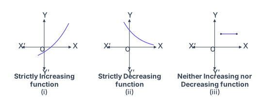
What Fig. 6.2 Shows

The figure presents three separate Cartesian plots side by side, each with labelled axes $X'\!-\!O\!-\!X$ (horizontal) and $Y'\!-\!O\!-\!Y$ (vertical). Every panel shares the same origin $O$ and arrow-headed axes, but each illustrates a different behaviour of a function as we move from left to right along the graph.

Panel (i) — Strictly Increasing function

A single indigo curve passes through the origin and rises continuously from the lower-left region to the upper-right region. As $x$ increases, $f(x)$ always increases — the graph never dips or flattens. This is the visual meaning of strictly increasing: for any two points $x_1 < x_2$ , we have $f(x_1) < f(x_2)$ .

Panel (ii) — Strictly Decreasing function

An indigo curve again passes through the origin, but now it falls continuously from the upper-left to the lower-right. As $x$ increases, $f(x)$ always decreases. For any $x_1 < x_2$ , we have $f(x_1) > f(x_2)$ .

Panel (iii) — Neither Increasing nor Decreasing

A short horizontal indigo segment sits in the first quadrant, with a solid slate dot at each endpoint. The function is constant on that interval — its value does not change as $x$ increases. Because it is neither rising nor falling, it belongs to neither of the first two categories.

Note

The horizontal segment in panel (iii) is the graphical counterpart of a constant function: $f(x) = c$ for all $x$ in that interval. The textbook later proves that if $f'(x) = 0$ everywhere on an interval, the function is constant there.

The Physical Idea

The core concept is simple: the direction of a graph as we scan it from left to right tells us whether the function is increasing, decreasing, or constant. This geometric intuition is the foundation for the analytical definitions given in the section:

Strictly increasing on $I$ : $x_1 < x_2 \;\Rightarrow\; f(x_1) < f(x_2)$ for all $x_1, x_2 \in I$ .
Strictly decreasing on $I$ : $x_1 < x_2 \;\Rightarrow\; f(x_1) > f(x_2)$ for all $x_1, x_2 \in I$ .
Constant on $I$ : $f(x) = c$ for all $x \in I$ .

The figure makes these abstract definitions immediately visible. Once you can see increase and decrease, the next step is to connect them to the sign of the derivative.

The Key Formula Developed from This Figure

The textbook uses the visual idea of Fig. 6.2 to motivate the first derivative test for monotonicity. The central result is Theorem 1:

f

Here $f'(x)$ denotes the derivative of $f$ at $x$ , and the interval $(a,b)$ is the open interval between $a$ and $b$ . The proof uses the Mean Value Theorem: if $x_1 < x_2$ in $[a,b]$ , there exists some $c$ between them such that

f(x_2) - f(x_1) = f'(c)(x_2 - x_1).

Since $x_2 - x_1 > 0$ , the sign of $f(x_2) - f(x_1)$ matches the sign of $f'(c)$ . A positive derivative forces $f(x_2) > f(x_1)$ (increasing), a negative derivative forces $f(x_2) < f(x_1)$ (decreasing), and a zero derivative forces $f(x_2) = f(x_1)$ (constant).

Watch out

The theorem requires $f'(x) > 0$ (or $<0$ ) for every $x$ in the open interval. A single point where the derivative is zero does not break monotonicity — for example, $f(x) = x^3$ has $f'(0) = 0$ but is still strictly increasing on $\mathbb{R}$ . The condition must hold on the whole interval, not just at isolated points.

How the Figure Connects to the Derivative …

Start your 14-day free trial to unlock the full solution →

← Previous · 6.2Q18 — Find the value of the following: The total revenue in Rupees received …Next · 6.3 →Example 7 — Show that the function given by f(x) = 7x - 3 is increasing on mathbbR…