Mathematics · Ch 5 — Continuity and Differentiability
Continuity
Continuity
5.2 Continuity
Understanding Continuity Through Examples
Before we formalise the idea, consider two simple functions that illustrate what it means for a function to fail to be continuous at a point.
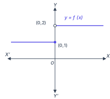
First example. Define
This function is defined at every real number. Its graph shows that for points near on the left — say , , — the function value is . For points near on the right — , , — the value is . The left-hand limit at is , the right-hand limit is , and these do not match. The function value at is , which equals the left-hand limit but not the right-hand limit. If you try to draw this graph, you must lift your pen when you reach from the left. This is a function that is not continuous at .
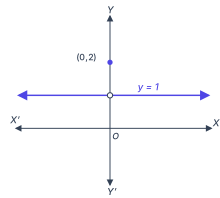
Second example. Now consider
Here both the left-hand and right-hand limits at equal . But the function value at is , which does not match the common limit. Again, drawing the graph forces you to lift your pen at . This is another instance of discontinuity at .
Informally, a function is continuous at a point if you can draw its graph near that point without lifting your pen. The precise mathematical definition captures this idea using limits.
Making the Idea Precise
We now turn this intuition into a precise statement. A function is continuous at a point of its domain when the limit of as exists and equals the value of the function there, ; and is a continuous function when it is continuous at every point of its domain. The full statements — the three conditions that must hold at a point, and how continuity is read at the endpoints of a closed interval — are set out in Definition 1 and Definition 2.
If any of the required conditions fails at , then is discontinuous at , and is called a point of discontinuity of .
Behaviour Near Zero — The Concept of Infinite Limits
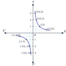
For , let us examine what happens as approaches . Tabulating the values for positive near (see Table 5.1) shows that as gets closer to from the right, grows without bound. We write
read as "the right-hand limit of at is plus infinity". Doing the same for negative near (see Table 5.2) shows that as approaches from the left, becomes arbitrarily negative:
…
Definition of Continuity at a Point
Let be a real function defined on a subset of , and let be a point in the domain of .
Then is continuous at if:
More elaborately, this means all three of the following conditions hold:
- is defined — the function has a value at .
- exists — both the left-hand limit and the right-hand limit exist and are equal.
- The limit equals the function value — .
If any of these fails, is discontinuous at , and is called a point of discontinuity.
Intuition
A function is continuous at a point if you can draw its graph without lifting your pen near that point — there is no sudden jump, hole, or break.
Tiny Concrete Example
Let . At : …
Definition of Continuity (Global)
A real function is said to be continuous if it is continuous at every point in its domain.
This means:
- For every point in the domain of , the condition
must hold.
- Equivalently, at each , the left-hand limit, right-hand limit, and the value of the function must all exist and be equal.
Special cases for closed intervals :
- At the left endpoint , continuity means .
- At the right endpoint , continuity means .
- Limits from outside the interval do not apply.
If the domain is a single point, the function is automatically continuous there.
Intuition
A function is continuous if you can draw its entire graph without lifting your pen — no breaks, jumps, or holes anywhere in the domain.
--- …
Drawn by us to help you understand the concept clearly, and verified to make sure it's accurate. For exams, practice from your textbook's own diagram.
Fig 5.1 is the first visual the textbook uses to introduce the idea of continuity. It plots a simple step function on the standard / Cartesian axes, with the origin labelled . The function is defined piecewise:
The graph shows two horizontal line segments. For , there is an indigo segment at height that ends with a solid dot at the point — this dot means the function actually takes the value at . For , a separate indigo segment sits at height , but it begins with an open circle at — that open circle tells you the function does not take the value at ; the point is not on the graph. The two levels do not meet; there is a clear vertical gap, a jump, at .
The physical idea is immediate: as you move along the -axis from left to right, the function's value stays at until you reach , then it suddenly leaps to . If you try to draw this graph with a pen, you must lift the pen off the paper at to jump from the lower segment to the upper one — you cannot trace the whole curve in one continuous stroke. That lifting of the pen is the intuitive signal that the function is not continuous at .
The textbook uses this figure to ground the formal definition of continuity. It observes that the left-hand limit of at is (because points like all give ), while the right-hand limit is (points like give ). Since these two one-sided limits are different, the ordinary limit does not exist. The value of the function at is , which happens to equal the left-hand limit but not the right-hand limit. The formal condition for continuity at a point is:
Equivalently, all three numbers — left-hand limit, right-hand limit, and the function value — must exist and be equal. Here, the left-hand limit () and right-hand limit () are unequal, so the limit does not exist, and the equality fails. Hence is discontinuous at , and is called a point of discontinuity. …
Drawn by us to help you understand the concept clearly, and verified to make sure it's accurate. For exams, practice from your textbook's own diagram.
Fig 5.2 is a simple but powerful picture of a function that is defined at every point yet still fails to be continuous. The axes are the standard Cartesian axes with origin O. A single horizontal line at stretches across the entire width of the graph, with arrowheads at both ends to show it continues indefinitely. But this line is broken: there is an open circle (a hole) at the point . Separately, a solid dot sits directly above that hole at .
The function being graphed is
The horizontal line at represents all points where — every real number except zero gives an output of 1. The open circle at tells you that the function does not take the value 1 at , even though the points arbitrarily close to 0 from both sides do. The solid dot at is the actual value of the function at : .
The physical idea is that the left-hand limit and the right-hand limit both exist and are equal — both are 1 — but the function's value at the point is different. The common limit exists (), yet . This is a removable discontinuity: you could "fix" the function by redefining to be 1, and the graph would become a continuous horizontal line. The hole-and-dot picture makes this instantly visible — the function jumps up to 2 at exactly one isolated point.
A common mistake is to think that if the left and right limits are equal, the function must be continuous. Fig 5.2 shows this is false: the limits can match, but if the function value at that point is different, continuity fails. The definition requires , not just that the limit exists.
The key formula the textbook develops with this figure is the formal definition of continuity at a point: …
Drawn by us to help you understand the concept clearly, and verified to make sure it's accurate. For exams, practice from your textbook's own diagram.
Fig 5.3 is the graph of the reciprocal function , drawn for . The plot has two separate hyperbolic branches, one in the first quadrant and one in the third quadrant, each shown in indigo. The horizontal axis is the -axis and the vertical axis is the -axis. On the -axis, ticks are marked at and .
The first-quadrant branch passes through the points , , , and . As increases beyond , the curve falls toward the -axis without ever touching it. As approaches from the right, the curve rises steeply toward the -axis, again without touching it. The third-quadrant branch is the mirror image through the origin: it passes through , , , and . As moves leftward from , the curve approaches the -axis from below; as approaches from the left, the curve plunges downward toward the -axis.
The central idea this figure teaches is the behaviour of a function near a point where it is not defined — here, . The textbook uses the graph to illustrate the concepts of infinite limits. As gets closer to from the right, the value of grows without bound. In symbols:
As approaches from the left, the value becomes arbitrarily negative:
Neither nor is a real number. These statements mean that the limit does not exist as a finite real number — the function simply grows or decreases without bound. Do not treat as a number you can do arithmetic with.
The figure also makes clear that the -axis () and the -axis () are asymptotes: the curve gets arbitrarily close to each axis but never crosses it. This is the geometric reason why is continuous at every point in its domain (all real numbers except ), but has a vertical asymptote at where it is not defined and therefore not continuous.
…
| | | | | | | | |
|---|---|---|---|---|---|---|---| …
| | | | | | | | |
|---|---|---|---|---|---|---|---| …