Mathematics · Ch 11 — Three-Dimensional Geometry

Angle Between Two Lines

11.4

Angle Between Two Lines

When two lines lie in space, they may intersect, be parallel, or be skew. The angle between them is the acute angle between their direction vectors.

The Fundamental Formula

Consider two lines through the origin with direction ratios $a_1, b_1, c_1$ and $a_2, b_2, c_2$ . Taking a point $P$ on the first and $Q$ on the second, $\overrightarrow{OP}$ and $\overrightarrow{OQ}$ are the direction vectors. If $\theta$ is the acute angle between them, the dot product gives:

\cos \theta = \frac{a_1 a_2 + b_1 b_2 + c_1 c_2}{\sqrt{a_1^2 + b_1^2 + c_1^2} \sqrt{a_2^2 + b_2^2 + c_2^2}}

The numerator is the dot product of the two direction vectors; the denominator is the product of their magnitudes.

Expression for $\sin \theta$

Using $\sin^2 \theta = 1 - \cos^2 \theta$ , the angle can also be written in terms of sine:

\sin \theta = \frac{\sqrt{(a_1 b_2 - a_2 b_1)^2 + (b_1 c_2 - b_2 c_1)^2 + (c_1 a_2 - c_2 a_1)^2}}{\sqrt{a_1^2 + b_1^2 + c_1^2} \sqrt{a_2^2 + b_2^2 + c_2^2}}

The numerator is the magnitude of the cross product of the direction vectors, from the identity $(a_1^2 + b_1^2 + c_1^2)(a_2^2 + b_2^2 + c_2^2) - (a_1 a_2 + b_1 b_2 + c_1 c_2)^2 = (a_1 b_2 - a_2 b_1)^2 + (b_1 c_2 - b_2 c_1)^2 + (c_1 a_2 - c_2 a_1)^2$ .

Note

The $\sin \theta$ formula is useful for checking parallel lines, since $\sin 0 = 0$ .

When Lines Do Not Pass Through the Origin

If the given lines do not pass through the origin, consider lines parallel to them that pass through the origin. Since parallel lines have the same direction, the angle is unchanged, so the same formulas apply using the original direction ratios.

Using Direction Cosines

Let $l_1, m_1, n_1$ and $l_2, m_2, n_2$ be the direction cosines of the two lines. Since $l_1^2 + m_1^2 + n_1^2 = 1$ and $l_2^2 + m_2^2 + n_2^2 = 1$ , the denominator becomes $1$ :

\cos \theta = |l_1 l_2 + m_1 m_2 + n_1 n_2|

The absolute value ensures the acute angle. Similarly, for the sine:

\sin \theta = \sqrt{(l_1 m_2 - l_2 m_1)^2 + (m_1 n_2 - m_2 n_1)^2 + (n_1 l_2 - n_2 l_1)^2}

Conditions for Perpendicular and Parallel Lines

Important

Perpendicular lines: with direction ratios $a_1, b_1, c_1$ and $a_2, b_2, c_2$ ,

$a_1 a_2 + b_1 b_2 + c_1 c_2 = 0$

This follows from $\theta = 90^\circ$ , where $\cos 90^\circ = 0$ .

Important

Parallel lines:

$\frac{a_1}{a_2} = \frac{b_1}{b_2} = \frac{c_1}{c_2}$

This follows from $\theta = 0$ , where $\sin 0 = 0$ forces each term $(a_1 b_2 - a_2 b_1)$ , $(b_1 c_2 - b_2 c_1)$ , $(c_1 a_2 - c_2 a_1)$ to vanish. …

Figure 11.4Two directed lines L1 and L2 through the origin O with points P and Q on them, enclosing the acute angle theta between the segments OP and OQ on the X, Y, Z axes.

Fig. 11.4 — Two directed lines L1 and L2 through the origin O with points P and Q on them, enclosing the acute angle theta between the segments OP and OQ on the X, Y, Z axes.

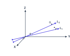
Drawn by us to help you understand the concept clearly, and verified to make sure it's accurate. For exams, practice from your textbook's own diagram.

Fig 11.4 is the geometric heart of the angle-between-lines concept. It shows a standard three-dimensional coordinate frame with axes X, Y, Z meeting at the origin O, drawn in an oblique perspective so all three axes are visible. Through O, two directed lines L₁ and L₂ are drawn, both extending into the first octant (where all coordinates are positive). The lines are coloured indigo and each has arrows on both ends — meaning they are considered as full lines through O, not just rays. L₂ is drawn above L₁, so the two lines are distinct and not coincident.

A point P is marked on L₁ and a point Q on L₂. The directed segments OP and OQ are then the vectors along the two lines. At O, a small arc is drawn between OP and OQ, and this arc is labelled θ — the acute angle between the two lines. The figure makes clear that θ is the smaller angle between the two directed lines, always taken between 0° and 90°.

The physical idea is simple: two lines through the origin have a well-defined angle between them, and that angle can be computed from the direction ratios (or direction cosines) of the lines. The figure anchors the vector approach — OP and OQ are vectors with components (a₁, b₁, c₁) and (a₂, b₂, c₂) respectively, so the angle between them comes directly from the dot product formula.

\cos \theta = \frac{a_1 a_2 + b_1 b_2 + c_1 c_2}{\sqrt{a_1^2 + b_1^2 + c_1^2} \;\sqrt{a_2^2 + b_2^2 + c_2^2}}

Here (a₁, b₁, c₁) and (a₂, b₂, c₂) are the direction ratios of L₁ and L₂. The denominator is the product of the magnitudes of the two direction vectors. The formula gives the cosine of the acute angle — the absolute value is taken if the dot product turns out negative, because θ is defined as the acute angle.

The textbook also derives an expression for sin θ:

\sin \theta = \frac{\sqrt{(a_1 b_2 - a_2 b_1)^2 + (b_1 c_2 - b_2 c_1)^2 + (c_1 a_2 - c_2 a_1)^2}}{\sqrt{a_1^2 + b_1^2 + c_1^2} \;\sqrt{a_2^2 + b_2^2 + c_2^2}}

This form is useful when you need the sine directly, or when checking perpendicularity (sin θ = 1) or parallelism (sin θ = 0). The numerator is the magnitude of the cross product of the two direction vectors.

Watch out

The figure shows lines through the origin, but the formulas work for any two lines in space. If the lines do not pass through the origin, simply translate them parallel to themselves so they both pass through O — the angle between them is unchanged. The direction ratios remain the same under translation. …

Start your 14-day free trial to unlock the full solution →

← Previous · 11.3.1Example 6 — Find the vector and the Cartesian equations of the line through the po…Next · 11.4 →Example 7 — Find the angle between the pair of lines given by vecr = 3hati + 2hatj…

Angle Between Two Lines