Physics · Ch 2 — Electrostatic Potential and Capacitance

Potential Due to a System of Charges

2.5

Potential Due to a System of Charges

The electric potential at a point due to a collection of point charges is simply the algebraic sum of the potentials due to each individual charge. This follows from the superposition principle, which applies to potential because it is a scalar quantity (unlike electric field, which is a vector).

Derivation for Discrete Charges

Consider $n$ point charges $q_1, q_2, \dots, q_n$ located at positions $\mathbf{r}_1, \mathbf{r}_2, \dots, \mathbf{r}_n$ relative to an origin. For a point P with position vector $\mathbf{r}$ , the potential $V_1$ at P due to $q_1$ alone is:

V_1 = \frac{1}{4\pi\varepsilon_0} \frac{q_1}{r_{1P}}

where $r_{1P} = |\mathbf{r} - \mathbf{r}_1|$ is the distance between $q_1$ and P. Similarly, for $q_2$ and $q_3$ :

V_2 = \frac{1}{4\pi\varepsilon_0} \frac{q_2}{r_{2P}}, \quad V_3 = \frac{1}{4\pi\varepsilon_0} \frac{q_3}{r_{3P}}

and so on for all charges. By superposition, the total potential $V$ at P is:

V = V_1 + V_2 + \dots + V_n

V = \frac{1}{4\pi\varepsilon_0} \left( \frac{q_1}{r_{1P}} + \frac{q_2}{r_{2P}} + \dots + \frac{q_n}{r_{nP}} \right)

This is the key formula for the potential due to a system of point charges. The sum is algebraic — signs of charges matter.

Continuous Charge Distribution

If the charge is distributed continuously (with volume charge density $\rho(\mathbf{r})$ ), we divide the distribution into small volume elements $\Delta v$ , each carrying charge $\rho \Delta v$ . The potential due to each element is:

\Delta V = \frac{1}{4\pi\varepsilon_0} \frac{\rho \Delta v}{r}

where $r$ is the distance from the element to the point P. Summing (integrating) over all elements gives the total potential:

V = \frac{1}{4\pi\varepsilon_0} \int \frac{\rho(\mathbf{r}')}{|\mathbf{r} - \mathbf{r}'|} \, dv'

Special Case: Uniformly Charged Spherical Shell

For a spherical shell of radius $R$ with total charge $q$ :

Outside the shell ( $r \geq R$ ): The potential is the same as if all charge were concentrated at the centre:

V = \frac{1}{4\pi\varepsilon_0} \frac{q}{r} \quad (r \geq R)

Inside the shell ( $r < R$ ): The electric field is zero, so no work is done moving a charge inside. Hence the potential is constant and equal to its value at the surface:

V = \frac{1}{4\pi\varepsilon_0} \frac{q}{R} \quad (r < R)

Example: Finding Points of Zero Potential …

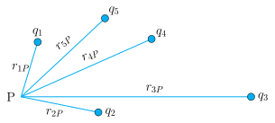
Figure 2.6Potential at a point due to a system of charges is the sum of potentials due to individual charges.

Fig. 2.6 — Potential at a point due to a system of charges is the sum of potentials due to individual charges.

Drawn by us to help you understand the concept clearly, and verified to make sure it's accurate. For exams, practice from your textbook's own diagram.

What the figure shows

The diagram is a schematic sketch of a point P (on the left) and five point charges $q_1, q_2, q_3, q_4, q_5$ scattered on the right. From P, five straight line segments fan out, each ending at one of the charges. Each segment is labelled with the corresponding distance: $r_{1P}, r_{2P}, r_{3P}, r_{4P}, r_{5P}$ . The charge $q_3$ is farthest to the right, so its segment $r_{3P}$ is the longest and nearly horizontal. The charge $q_2$ is nearest to P, located below and to the right. Charges $q_4$ and $q_5$ cluster together in the upper-right region, while $q_1$ is in the upper-right direction. All five segments share the common vertex at P.

Physical idea

The figure illustrates the superposition principle for electrostatic potential. The total electric potential at a point due to a collection of point charges is simply the algebraic sum of the potentials produced by each charge individually. Unlike electric field (which is a vector and requires vector addition), potential is a scalar — so you just add the numbers, taking care of signs.

Key formula developed with this figure

The textbook uses this figure to derive the general expression for the potential at P due to $n$ point charges:

V = V_1 + V_2 + \dots + V_n = \frac{1}{4\pi\varepsilon_0} \left( \frac{q_1}{r_{1P}} + \frac{q_2}{r_{2P}} + \dots + \frac{q_n}{r_{nP}} \right)

where:

$V$ is the total electric potential at point P (in volts)
$\frac{1}{4\pi\varepsilon_0}$ is Coulomb's constant ( $\varepsilon_0$ = permittivity of free space)
$q_1, q_2, \dots, q_n$ are the source charges (in coulombs) …

Start your 14-day free trial to unlock the full solution →

← Previous · 2.4Potential Due to an Electric Dipole Next · 2.5 →Example 2.2 — Two charges 3 × 10⁻⁸C and -2 × 10⁻⁸C are located 15cm apart. At what p…