Economics · Ch 10 — The Theory of the Firm under Perfect Competition

Long Run Supply Curve of a Firm

10.4.2

Long Run Supply Curve of a Firm

The long run supply curve of a firm under perfect competition is derived from its long run cost curves. Unlike the short run, where the firm faces fixed costs, in the long run all inputs are variable and the firm can choose any plant size. The key curves here are the long run marginal cost (LRMC) curve and the long run average cost (LRAC) curve.

The derivation proceeds in two parts, exactly as it did for the short run. First, we determine what the firm does when the market price is high enough to cover its long run average costs. Then we examine the case when the price is too low.

Case 1: Price Greater Than or Equal to the Minimum LRAC

Consider a market price $p_1$ that lies above the minimum point of the LRAC curve. The firm, being a profit-maximiser, will equate this price with its long run marginal cost. It finds the output level $q_1$ where $p_1 = LRMC$ on the rising portion of the LRMC curve.

At this output $q_1$ , the LRAC is less than or equal to the market price $p_1$ . This means all three conditions for long run profit maximisation are satisfied:

Price equals LRMC (the first-order condition).
LRMC is rising at the point of intersection (the second-order condition ensures it is a maximum, not a minimum).
Price is at least as large as LRAC (so the firm is not making a loss).

Therefore, when the market price is $p_1$ , the firm supplies output $q_1$ in the long run. This is a positive, profitable level of production.

Case 2: Price Less Than the Minimum LRAC

Now suppose the market price is $p_2$ , which is below the minimum point of the LRAC curve. The firm faces a problem. Condition 3 from the profit-maximisation rules states that if a firm produces a positive output in the long run, the market price must be greater than or equal to the LRAC at that output. Otherwise, the firm would be making a loss on every unit produced.

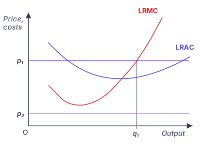
Looking at Figure 4.9, for every positive output level, the LRAC curve lies strictly above $p_2$ . There is simply no output at which the firm can cover its average costs. The firm cannot reduce its plant size or adjust inputs to bring costs down to the price level — the minimum LRAC itself is already above the price.

Figure 4.9Profit maximisation in the Long Run for Different Market Price Values. The figure shows the output levels chosen by a profit-maximising firm in the long run for two values of the market price: p₁ and p₂. When the market price is p₁, the output level of the firm is q₁; when the market price is p₂, the firm produces zero output.

Fig. 4.9 — Profit maximisation in the Long Run for Different Market Price Values. The figure shows the output levels chosen by a profit-maximising firm in the long run for two values of the market price: p₁ and p₂. When the market price is p₁, the output level of the firm is q₁; when the market price is p₂, the firm produces zero output.

Drawn by us to help you understand the concept clearly, and verified to make sure it's accurate. For exams, practice from your NCERT textbook's own diagram.

The figure plots the market price $p$ on the vertical axis and the firm’s output $q$ on the horizontal axis. Two horizontal lines are drawn at heights $p_1$ and $p_2$ , representing two different market prices that the firm takes as given. The firm’s long-run marginal cost curve $LMC$ slopes upward, and its long-run average cost curve $LAC$ is U-shaped. The key feature is that the $LMC$ curve cuts the $LAC$ curve at the minimum point of $LAC$ — call that point $M$ , with coordinates $(q^*, p^*)$ .

When the market price is $p_1$ , which lies above the minimum of $LAC$ , the firm chooses output $q_1$ where the horizontal price line $p = p_1$ intersects the $LMC$ curve from below. At $q_1$ , price equals long-run marginal cost: $p_1 = LMC(q_1)$ . Because $p_1$ exceeds the average cost at $q_1$ , the firm earns positive economic profit. The vertical distance between the price line and the $LAC$ curve at $q_1$ is the per-unit profit, and the rectangle with height $p_1 - LAC(q_1)$ and width $q_1$ shows total profit.

When the market price falls to $p_2$ , which is below the minimum of $LAC$ , no positive output can yield a non-negative profit. The firm would minimise its loss by producing zero output — it shuts down in the long run. The figure shows this by having no intersection between the $p_2$ line and the $LMC$ curve at any output where price covers average cost. The firm’s long-run supply curve is therefore the portion of the $LMC$ curve that lies above the minimum of $LAC$ .

\text{Long-run profit-maximising condition: } p = LMC(q), \text{ provided } p \ge \min LAC

The physical idea is that in the long run, all inputs are variable, so the firm can exit the industry entirely. It will produce only if the market price is at least as high as the lowest possible average cost — the break-even price. If price falls below that floor, the firm cannot cover its average cost at any output and shuts down, producing zero. …

Watch out

A common mistake is to think the firm might produce a small amount to "cover variable costs" in the long run. In the long run, there are no fixed costs — all costs are variable. If price is below LRAC at every output, the firm loses money on every unit it produces. The rational choice is to produce zero.

The firm's profit-maximising decision is therefore to produce zero output. It shuts down completely in the long run.

The Long Run Supply Curve

Combining the two cases gives the complete long run supply curve of a perfectly competitive firm.

For any market price below the minimum LRAC, the firm supplies zero output.
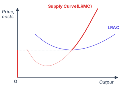
For any market price equal to or above the minimum LRAC, the firm supplies the output where price equals LRMC on the rising portion of the LRMC curve. …

Figure 4.10The Long Run Supply Curve of a Firm. The long run supply curve of a firm, which is based on its long run marginal cost curve (LRMC) and long run average cost curve (LRAC), is represented by the bold line.

Fig. 4.10 — The Long Run Supply Curve of a Firm. The long run supply curve of a firm, which is based on its long run marginal cost curve (LRMC) and long run average cost curve (LRAC), is represented by the bold line.

Drawn by us to help you understand the concept clearly, and verified to make sure it's accurate. For exams, practice from your NCERT textbook's own diagram.

The figure plots two curves on a standard pair of axes. The horizontal axis measures the quantity of output, $q$ , and the vertical axis measures cost and revenue in rupees. The two curves are the long-run marginal cost curve, labelled LRMC, and the long-run average cost curve, labelled LRAC. Both are drawn as U-shaped curves, with LRMC intersecting LRAC at the minimum point of LRAC. The bold line that forms the firm’s long-run supply curve is not a separate curve but a specific segment of the LRMC curve: it is the portion of LRMC that lies above the minimum point of LRAC. The part of LRMC below that minimum is shown as a thin line, indicating it is not part of the supply curve.

The physical idea is straightforward. In the long run, a firm can adjust all its inputs, so it chooses the plant size that minimises average cost for any given output. The firm will produce only if the market price covers the minimum possible average cost; otherwise it shuts down permanently. The minimum point of LRAC is therefore the firm’s break-even price — the lowest price at which it can survive in the long run. For any price above that minimum, the firm maximises profit by producing the quantity where price equals LRMC. Hence the long-run supply curve is the upward-sloping part of LRMC starting from the shut-down/break-even point.

The key formula the textbook develops with this figure is the long-run profit-maximisation condition and the break-even condition. For a perfectly competitive firm in the long run:

P = LRMC(q) \quad \text{and} \quad P \geq \min LRAC

Here $P$ is the market price (which the firm takes as given), $LRMC(q)$ is the long-run marginal cost at output $q$ , and $\min LRAC$ is the minimum value of the long-run average cost curve. The firm chooses $q$ such that price equals LRMC, but only if that price is at least as high as the lowest possible average cost. If $P < \min LRAC$ , the firm exits the industry entirely — its long-run supply is zero. …

Start your 14-day free trial to unlock the full solution →

← Previous · 10.4.1Short Run Supply Curve of a Firm Next · 10.4.3 →The Shut Down Point