Mathematics · Ch 12 — Linear Programming

Graphical Method of Solving Linear Programming Problems

12.2.2

Graphical Method of Solving Linear Programming Problems

12.2.2 Graphical Method of Solving Linear Programming Problems

From Inequalities to Optimization

In Class XI you learned to graph a system of linear inequalities in two variables and find the solution region. The graphical method for linear programming builds directly on that skill — but instead of just finding where all constraints are satisfied, we search that region for the point giving the best (maximum or minimum) value of a linear objective function.

Revisit the investment problem from Section 12.2:

\begin{aligned} 5x + y &\leq 100 \quad \text{(1)} \\ x + y &\leq 60 \quad \text{(2)} \\ x &\geq 0 \quad \text{(3)} \\ y &\geq 0 \quad \text{(4)} \end{aligned}

where $x$ = number of tables and $y$ = number of chairs. The objective is to maximize profit $Z = 250x + 75y$ .

The Feasible Region

Graphing all four inequalities, the shaded region common to all half-planes is the feasible region — in Fig 12.1 of the textbook, the quadrilateral OABC.

Feasible region: The common region determined by all constraints (including $x \geq 0$ , $y \geq 0$ ) of a linear programming problem.

Every point inside or on the boundary is a feasible solution — for example (10, 50), (0, 60), (20, 0). Any point outside, such as (25, 40), is an infeasible solution.

Watch out

Points on the boundary are also feasible — they satisfy the constraints as equalities. It is a mistake to think only points strictly inside the region are feasible.

The Challenge: Finding the Optimal Point

The feasible region contains infinitely many points, so we cannot check each one. Two fundamental theorems (stated here without proof) solve this problem.

Theorem 1: The Corner Point Principle

Important

Theorem 1: Let $R$ be the feasible region for a linear programming problem, and $Z = ax + by$ the objective function. When $Z$ has an optimal value (maximum or minimum), this value must occur at a corner point (vertex) of $R$ .

A corner point is where two boundary lines intersect. So instead of checking every point, we only examine the vertices.

Theorem 2: Existence of Optima for Bounded Regions

Important

Theorem 2: If the feasible region $R$ is bounded (can be enclosed within a circle), then $Z$ has both a maximum and a minimum value on $R$ , each occurring at a corner point of $R$ .

Note

If $R$ is unbounded (extends indefinitely), a maximum or minimum may not exist. However, if an optimal value does exist, it still occurs at a corner point (by Theorem 1).

The Corner Point Method

Find the feasible region and its corner points, by inspection or by solving the equations of the intersecting lines at each vertex.
Evaluate $Z = ax + by$ at each corner point. Let $M$ be the largest value and $m$ the smallest.
Determine optimal values:
- (i) If $R$ is bounded, $M$ is the maximum value and $m$ the minimum value of $Z$ .
- (ii) If $R$ $R$ is unbounded:
  - (a) $M$ is the maximum value if and only if the open half-plane $ax + by > M$ has no point in common with $R$ ; otherwise $Z$ has no maximum.
  - (b) $m$ is the minimum value if and only if the open half-plane $ax + by < m$ has no point in common with $R$ ; otherwise $Z$ has no minimum.

Tip

The extra check for unbounded regions is crucial: even if a corner point gives the smallest value among all vertices, a point elsewhere in the region might give an even smaller value. …

Theorem 1

Theorem 2: The Corner-Point Theorem for Bounded Feasible Regions

Statement (from NCERT Class 12):

Let $R$ be the feasible region for a linear programming problem, and let $Z = ax + by$ be the objective function. If $R$ is bounded, then the objective function $Z$ has both a maximum and a minimum value on $R$ , and each of these occurs at a corner point (vertex) of $R$ .

What the hypotheses mean

Feasible region $R$ is the set of all points $(x, y)$ that satisfy every constraint (including $x \geq 0, y \geq 0$ ). Graphically, it is the common shaded region formed by all the half-planes.
Bounded means the region can be enclosed inside some circle of finite radius. In other words, it does not stretch off to infinity in any direction. A bounded feasible region is always a convex polygon (or a line segment, or a single point).
Objective function $Z = ax + by$ is a linear function whose value we want to maximise or minimise.

Important

The theorem guarantees both a maximum and a minimum exist when the region is bounded. This is not true for unbounded regions — there, a maximum or minimum may not exist at all.

Complete Proof

›Proof

Step 1: The feasible region is a closed, bounded convex polygon.

Since $R$ is defined by a finite set of linear inequalities, its boundary consists of straight line segments. Because $R$ is bounded, it has a finite number of corner points (vertices). Let these vertices be $V_1, V_2, \dots, V_k$ .

Step 2: Any point in $R$ can be expressed as a convex combination of the vertices.

This is a property of convex polygons: every point $P$ inside or on the boundary of $R$ can be written as

$P = \lambda_1 V_1 + \lambda_2 V_2 + \dots + \lambda_k V_k$

where $\lambda_i \geq 0$ for all $i$ and $\lambda_1 + \lambda_2 + \dots + \lambda_k = 1$ .

Step 3: Evaluate $Z$ at such a point.

Since $Z = ax + by$ is linear, we have:

$Z(P) = a x_P + b y_P = a\left(\sum_{i=1}^k \lambda_i x_i\right) + b\left(\sum_{i=1}^k \lambda_i y_i\right)$

$= \sum_{i=1}^k \lambda_i (a x_i + b y_i) = \sum_{i=1}^k \lambda_i Z(V_i)$

So the value of $Z$ at any point $P$ is a weighted average of its values at the vertices, with the same weights $\lambda_i$ .

Step 4: The maximum of $Z$ occurs at a vertex.

Let $M = \max\{Z(V_1), Z(V_2), \dots, Z(V_k)\}$ be the largest value among the vertices. Then for any point $P$ in $R$ :

$Z(P) = \sum_{i=1}^k \lambda_i Z(V_i) \leq \sum_{i=1}^k \lambda_i M = M \sum_{i=1}^k \lambda_i = M$

Therefore, no point in $R$ can give a value larger than $M$ . Since $M$ is actually attained at some vertex (by definition), the maximum value of $Z$ on $R$ is exactly $M$ , and it occurs at that vertex.

Step 5: The minimum of $Z$ occurs at a vertex.

Let $m = \min\{Z(V_1), Z(V_2), \dots, Z(V_k)\}$ be the smallest value among the vertices. Then for any point $P$ in $R$ :

$Z(P) = \sum_{i=1}^k \lambda_i Z(V_i) \geq \sum_{i=1}^k \lambda_i m = m \sum_{i=1}^k \lambda_i = m$

So no point gives a value smaller than $m$ , and $m$ is attained at some vertex. Hence the minimum value is $m$ , occurring at a vertex.

Step 6: Both extremal values exist.

Because $R$ is bounded and closed, the continuous function $Z$ must attain both a maximum and a minimum on $R$ (by the Extreme Value Theorem from calculus). Steps 4 and 5 show these must be at vertices. This completes the proof.

When is this theorem used? …

Theorem 2

Theorem 2: The Corner-Point Theorem for Bounded Feasible Regions

Statement (from NCERT Class 12):

What the hypotheses mean

Feasible region $R$ is the set of all points $(x, y)$ that satisfy every constraint (including $x \geq 0, y \geq 0$ ). Graphically, it is the common shaded region formed by all the half-planes.
Bounded means the region can be enclosed inside some circle of finite radius. In other words, it does not stretch off to infinity in any direction. A bounded feasible region is always a convex polygon (or a line segment, or a single point).
Objective function $Z = ax + by$ is a linear function whose value we want to maximise or minimise.

Important

The theorem guarantees both a maximum and a minimum exist when the region is bounded. This is not true for unbounded regions — there, a maximum or minimum may not exist at all.

Complete Proof

›Proof

Step 1: The feasible region is a closed, bounded convex polygon.

Step 2: Any point in $R$ can be expressed as a convex combination of the vertices.

This is a property of convex polygons: every point $P$ inside or on the boundary of $R$ can be written as

$P = \lambda_1 V_1 + \lambda_2 V_2 + \dots + \lambda_k V_k$

where $\lambda_i \geq 0$ for all $i$ and $\lambda_1 + \lambda_2 + \dots + \lambda_k = 1$ .

Step 3: Evaluate $Z$ at such a point.

Since $Z = ax + by$ is linear, we have:

$Z(P) = a x_P + b y_P = a\left(\sum_{i=1}^k \lambda_i x_i\right) + b\left(\sum_{i=1}^k \lambda_i y_i\right)$

$= \sum_{i=1}^k \lambda_i (a x_i + b y_i) = \sum_{i=1}^k \lambda_i Z(V_i)$

So the value of $Z$ at any point $P$ is a weighted average of its values at the vertices, with the same weights $\lambda_i$ .

Step 4: The maximum of $Z$ occurs at a vertex.

Let $M = \max\{Z(V_1), Z(V_2), \dots, Z(V_k)\}$ be the largest value among the vertices. Then for any point $P$ in $R$ :

$Z(P) = \sum_{i=1}^k \lambda_i Z(V_i) \leq \sum_{i=1}^k \lambda_i M = M \sum_{i=1}^k \lambda_i = M$

Step 5: The minimum of $Z$ occurs at a vertex.

Let $m = \min\{Z(V_1), Z(V_2), \dots, Z(V_k)\}$ be the smallest value among the vertices. Then for any point $P$ in $R$ :

$Z(P) = \sum_{i=1}^k \lambda_i Z(V_i) \geq \sum_{i=1}^k \lambda_i m = m \sum_{i=1}^k \lambda_i = m$

So no point gives a value smaller than $m$ , and $m$ is attained at some vertex. Hence the minimum value is $m$ , occurring at a vertex.

Step 6: Both extremal values exist.

When is this theorem used? …

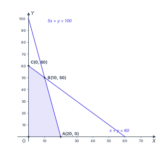
Figure 12.1A shaded bounded feasible region OABC in the first quadrant formed by the constraint lines 5x + y = 100 and x + y = 60, with corner points A(20, 0), B(10, 50) and C(0, 60) marked.

Fig. 12.1 — A shaded bounded feasible region OABC in the first quadrant formed by the constraint lines 5x + y = 100 and x + y = 60, with corner points A(20, 0), B(10, 50) and C(0, 60) marked.

Drawn by us to help you understand the concept clearly, and verified to make sure it's accurate. For exams, practice from your NCERT textbook's own diagram.

Fig 12.1 is the first graphical illustration of a linear programming problem in the chapter. It shows the feasible region for the tables-and-chairs investment problem, and it is the picture that makes the entire Corner Point Method intuitive.

The graph is drawn in the first quadrant only, because the non-negativity constraints $x \geq 0$ and $y \geq 0$ restrict everything to positive $x$ and $y$ . The horizontal axis is labelled $x$ (number of tables), and the vertical axis is $y$ (number of chairs). Two straight lines are drawn across this quadrant:

The indigo line $5x + y = 100$ cuts the $y$ -axis at $(0,100)$ and the $x$ -axis at $(20,0)$ .
The line $x + y = 60$ cuts the $y$ -axis at $(0,60)$ and the $x$ -axis at $(60,0)$ .

These two lines intersect at point $B$ , whose coordinates are $(10,50)$ . That intersection is the key — it is where both constraints are simultaneously tight.

The region that satisfies all four constraints — $5x + y \leq 100$ , $x + y \leq 60$ , $x \geq 0$ , $y \geq 0$ — is the polygon $OABC$ , shaded light indigo. Its vertices are:

$O(0,0)$ — the origin, where nothing is bought.
$A(20,0)$ — on the $x$ -axis, where $5x + y = 100$ meets the $x$ -axis.
$B(10,50)$ — the intersection of the two constraint lines.
$C(0,60)$ — on the $y$ -axis, where $x + y = 60$ meets the $y$ -axis.

Every point inside or on the boundary of this polygon is a feasible solution — a combination of tables and chairs that does not exceed the dealer's budget or storage capacity. Points outside, like $(25,40)$ , are infeasible because they violate at least one constraint.

Note

The feasible region is always a convex polygon. Here it is bounded (it can be enclosed in a circle), so both a maximum and a minimum value of the objective function exist, and they occur at corner points.

The objective function for this problem is the profit:

Z = 250x + 75y

where $x$ is the number of tables (profit ₹250 per table) and $y$ is the number of chairs (profit ₹75 per chair). The textbook evaluates $Z$ at each corner point:

Vertex	Coordinates	$Z = 250x + 75y$ (₹)
$O$	$(0,0)$	$0$
$A$	$(20,0)$	$5000$
$B$	$(10,50)$	$6250$ ← maximum
$C$	$(0,60)$	$4500$

Start your 14-day free trial to unlock the full solution →

← Previous · 12.2.1Mathematical Formulation of the Problem Next · 12.2.2 →Example 1 — Solve the following linear programming problem graphically: Maximise Z…