Mathematics · Ch 10 — Vector Algebra
Addition of Vectors
Addition of Vectors
10.4 Addition of Vectors
The Triangle Law of Vector Addition
When a girl moves from A to B, and then from B to C, her net displacement from A to C is the vector sum of the two individual displacements. This leads to the triangle law of vector addition.
To add two vectors and , place them so that the initial point of coincides with the terminal point of . The vector from the initial point of to the terminal point of is the sum .
In triangle ABC (Fig 10.8(ii)):
Thus the third side AC represents the resultant of the two vectors.
Zero Resultant from a Closed Triangle
If the sides of a triangle are taken in order, the resultant is zero because the initial and terminal points coincide (Fig 10.8(iii)):
Since , this gives the triangle law algebraically:
Vector Subtraction
To subtract from , construct (same magnitude, opposite direction). Then:
Applying the triangle law with :
The geometric picture of is correct, but always compute it algebraically as using the triangle law with the negative vector.
The Parallelogram Law of Vector Addition
A boat crossing a river has two velocities acting simultaneously — the engine velocity and the river-flow velocity — and its actual velocity is their resultant.
Parallelogram Law: If two vectors are represented by two adjacent sides of a parallelogram in magnitude and direction, then their sum is represented in magnitude and direction by the diagonal of the parallelogram through their common point.
In Fig 10.9, if and , then the diagonal through the common point A gives .
The parallelogram law and the triangle law are equivalent. From Fig 10.9, using the triangle law:
since (opposite sides of a parallelogram are equal and parallel).
Properties of Vector Addition
Property 1: Commutative Property
For any two vectors and :
›Proof
Consider parallelogram ABCD (Fig 10.10) with and .
In triangle ABC: .
Since opposite sides are equal and parallel, and .
In triangle ADC: .
Hence .
Property 2: Associative Property
For any three vectors , , and :
…
For any three vectors , , and , the scalar triple product satisfies:
.
This means the dot and cross operations can be swapped without changing the value, as long as the cyclic order is preserved. It is used to simplify expressions involving volume of a parallelepiped or …
For any three vectors , , and , the scalar triple product satisfies:
.
This means the dot and cross operations can be swapped without changing the value, as long as the cyclic order is preserved. It is used to simplify expressions involving volume of a parallelepiped or …
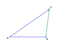
Drawn by us to help you understand the concept clearly, and verified to make sure it's accurate. For exams, practice from your NCERT textbook's own diagram.
Fig 10.7 is the simplest possible picture of vector addition — a triangle. The three vertices are labelled A (bottom-left), B (bottom-right), and C (top-right). The base AB runs horizontally from A to B. The side BC rises vertically from B to C, and the side AC is the diagonal from A to C.
The physical idea is a girl walking from A to B, then from B to C. Her net displacement — the straight-line path from start to finish — is the vector from A to C. The figure shows that the two successive displacements, AB and BC, combine to give the single displacement AC. This is the triangle law of vector addition: if you place two vectors so that the head of the first meets the tail of the second, their sum is the vector from the tail of the first to the head of the second.
The key formula the textbook develops from this figure is:
Here, is the vector from A to B (the first displacement), is the vector from B to C (the second displacement), and is their sum — the resultant vector from A to C.
The triangle law works for any two vectors, not just perpendicular ones. The figure uses a right-angled triangle for clarity, but the rule holds for any shape of triangle.
The textbook then generalises this. In Fig 10.8(ii), vector is placed so its tail coincides with the head of vector . The third side of the triangle, from the tail of to the head of , gives . This is the same idea as Fig 10.7, just with generic vectors instead of a specific path.
The triangle law is equivalent to the parallelogram law. In Fig 10.9, the diagonal of the parallelogram is the same sum as the third side of the triangle formed by the two adjacent sides. Both laws give the same resultant. …
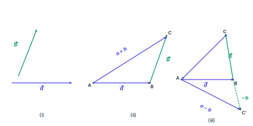
Drawn by us to help you understand the concept clearly, and verified to make sure it's accurate. For exams, practice from your NCERT textbook's own diagram.
Figure 10.8 is a three-panel diagram that builds the triangle law of vector addition from scratch, then extends it to subtraction. The textbook uses it to show why the triangle law works and how subtraction is just addition of a reversed vector.
Panel (i) shows the two vectors we start with: vector drawn horizontally to the right, and vector drawn at an angle (emerald in the original). They are separate, with no common point yet — this is the raw material before any operation.
Panel (ii) is the core of the triangle law. Vector is placed as the displacement from to (so ). Then vector is shifted — without changing its length or direction — so that its tail sits exactly at the head of , point . This gives . The third side of triangle , from to , is the resultant: . The physical idea is that if you go from to and then from to , the net displacement is the straight shot from to .
Panel (iii) introduces subtraction. Starting from the same triangle , a new point is constructed such that — that is, a vector with the same magnitude as but pointing in the opposite direction (drawn as a dashed arrow). Now applying the triangle law to and gives . This is the geometric meaning of vector subtraction: reverse the vector you want to subtract, then add.
A common mistake is to think points from the head of to the head of in the original triangle. That is not what the figure shows. The subtraction vector is , which uses a separate construction with the reversed vector.
The key formula developed from this figure is the triangle law of vector addition:
where , , and the resultant . The figure also leads to the corollary that when vectors are taken in order around a closed triangle, the sum is zero: , because the initial and terminal points coincide. This is visible in panel (ii) if you consider the full triangle — going brings you back to where you started.
The subtraction formula follows directly:
…
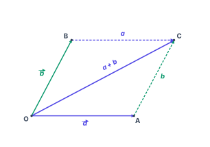
Drawn by us to help you understand the concept clearly, and verified to make sure it's accurate. For exams, practice from your NCERT textbook's own diagram.
What Fig 10.9 Shows
The figure is a clean parallelogram labelled OACB. The vector runs along the bottom edge from O to A — this is the base of the parallelogram, drawn as a solid arrow. The vector goes from O up the left side to B, shown as a solid arrow (the textbook marks it in emerald). From the common starting point O, these two vectors form the adjacent sides of the parallelogram.
The diagonal from O to C is the vector , drawn as a solid arrow. This diagonal represents the resultant — the single vector that has the same effect as applying and together. The remaining two sides are shown as dashed lines: BC is parallel to OA and equal in length to , and AC is parallel to OB and equal in length to .
The Physical Idea
The parallelogram law answers a practical question: if two forces, velocities, or displacements act on an object at the same time, what is the net effect? The boat example in the textbook makes this concrete — a boat heading straight across a river is simultaneously pushed downstream by the current. The boat's actual path is neither the direction it points nor the direction of the current, but the diagonal of the parallelogram formed by these two velocity vectors.
The key insight is that the diagonal through the common point O gives both the magnitude and direction of the resultant. This is not a guess — it follows directly from the triangle law of vector addition. If you travel from O to A (vector ) and then from A to C (vector ), you end up at C. The straight path from O to C is therefore .
The dashed sides BC and AC are not just decoration — they show that the parallelogram is really two triangles glued together. Triangle OAC gives by the triangle law, and triangle OBC gives . The fact that both diagonals are the same vector proves commutativity.
The Central Formula
The figure directly illustrates the parallelogram law of vector addition:
where:
- is the vector along the base (from O to A)
- is the vector up the left side (from O to B)
- is the diagonal from O to C, the resultant
The textbook also shows how the triangle law gives the same result. From triangle OAC:
But (opposite sides of a parallelogram are equal and parallel), so:
A common mistake is to think the diagonal from A to B also represents the sum. It does not — only the diagonal through the common starting point O gives . The other diagonal gives (or , depending on direction). …
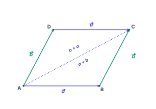
Drawn by us to help you understand the concept clearly, and verified to make sure it's accurate. For exams, practice from your NCERT textbook's own diagram.
Fig 10.10 is the parallelogram ABCD that the textbook uses to prove the commutative property of vector addition. The figure is a clean, labelled parallelogram with vertices A, B, C, D taken in order. The two adjacent sides from the common point A are labelled: side AB is vector a, and side AD is vector b. The opposite sides are equal and parallel — so DC is also a, and BC is also b. The two diagonals are drawn as dotted lines. The diagonal from A to C (the one through the interior) is labelled a + b. The other diagonal, from B to D, is labelled a − b on one side and b − a on the other — this shows that the two diagonals represent the sum and the difference of the two side vectors.
The physical idea is simple: if you walk from A to B (vector a) and then from B to C (vector b), you end up at C. The direct path from A to C is the sum a + b. But the figure also shows that if you instead go from A to D (vector b) and then from D to C (vector a), you still end up at C. That is the commutative law: a + b = b + a. The parallelogram makes this equality visually obvious — the two different routes to C give the same diagonal.
The key formula the textbook develops with this figure is the commutative property:
Here, a and b are any two vectors. In the figure, a = and b = . Using the triangle law in triangle ABC, we get . Using the triangle law in triangle ADC (where and ), we get . Since both expressions equal the same diagonal vector , the equality follows.
A common mistake is to think the diagonal from A to C equals a + b only when the vectors are perpendicular. That is false — the parallelogram law works for any two vectors placed tail-to-tail. The diagonal always gives the sum, regardless of the angle between them. …
Drawn by us to help you understand the concept clearly, and verified to make sure it's accurate. For exams, practice from your NCERT textbook's own diagram.
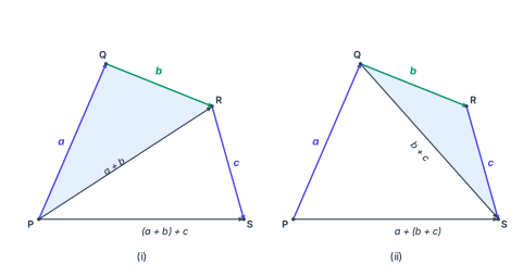
Figure 10.11 is the visual proof of the associative property of vector addition: for any three vectors , , ,
The figure has two panels, (i) and (ii), each showing the same four points — P, Q, R, S — arranged in a quadrilateral. The path from P to Q to R to S is the same in both panels; what changes is which diagonal is drawn first.
Panel (i) — grouping first.
The vector runs from P to Q, from Q to R, and from R to S. The diagonal from P to R is drawn and labelled (the triangle PQR is shaded to show this intermediate sum). Then the diagonal from P to S is drawn, representing — the resultant of first adding and , then adding to that sum.
Panel (ii) — grouping first.
The same vectors , , are placed identically. Now the diagonal from Q to S is drawn and labelled (triangle QRS is shaded). Then the diagonal from P to S is drawn again, this time representing — the resultant of first adding and , then adding to that sum.
The key point: the final diagonal PS is the same in both panels. The figure shows that no matter how you group the three vectors, the net displacement from P to S is identical. This is the associative law in action.
Here , , are any three vectors placed head-to-tail. The equality means that when adding vectors, brackets are unnecessary — you can write without ambiguity. …