Mathematics · Ch 13 — Probability

Partition of a Sample Space

13.5.1

Partition of a Sample Space

The Idea of a Partition

Rolling a die gives sample space $S = \{1,2,3,4,5,6\}$ . Consider:

$E_1$ : the outcome is even $\{2,4,6\}$
$E_2$ : the outcome is odd $\{1,3,5\}$

These have no common outcome ( $E_1 \cap E_2 = \phi$ ), together cover every outcome ( $E_1 \cup E_2 = S$ ), and each has positive probability ( $P(E_1) = P(E_2) = \frac12 > 0$ ). This is the simplest partition of a sample space — a way of cutting $S$ into non-overlapping pieces that together make up the whole, each with a chance of occurring.

Formal Definition of a Partition

A set of events $\{E_1, E_2, \dots, E_n\}$ is a partition of $S$ if:

Pairwise disjoint: $E_i \cap E_j = \phi$ for all $i \neq j$ — no two events share an outcome.
Exhaustive: $E_1 \cup E_2 \cup \dots \cup E_n = S$ — every outcome belongs to at least one event.
Positive probability: $P(E_i) > 0$ for every $i$ — each event has a non-zero chance.

Simple Partition Illustrations

Illustration 1: An event and its complement. For any event $E$ that is neither impossible nor certain, $\{E, E'\}$ is a partition of $S$ : $E \cap E' = \phi$ , $E \cup E' = S$ , and $P(E) > 0$ , $P(E') > 0$ .

Illustration 2: Four events from two events. For any two events $E$ and $F$ , the following form a partition of $S$ :

\{E \cap F',\; E \cap F,\; E' \cap F,\; E' \cap F'\}

Pairwise disjoint: any two involve opposite membership in $E/E'$ or $F/F'$ , e.g. $(E \cap F') \cap (E \cap F) = E \cap (F' \cap F) = \phi$ .
Exhaustive: every outcome is in $E$ or $E'$ and in $F$ or $F'$ , so it falls into exactly one combination.
Positive probability: each is assumed to have positive probability for the partition to be meaningful.

Note

A partition is not unique. For example $\{E, E'\}$ is one partition, while $\{E \cap F', E \cap F, E' \cap F, E' \cap F'\}$ is a finer one of the same $S$ .

Why Partitions Matter: The Theorem of Total Probability …

Figure 13.4The sample space S partitioned into mutually exclusive and exhaustive events E1, E2, E3, ..., En with an event A drawn as an oval cutting across the partition, illustrating Bayes' theorem.

Fig. 13.4 — The sample space S partitioned into mutually exclusive and exhaustive events E1, E2, E3, ..., En with an event A drawn as an oval cutting across the partition, illustrating Bayes' theorem.

Drawn by us to help you understand the concept clearly, and verified to make sure it's accurate. For exams, practice from your textbook's own diagram.

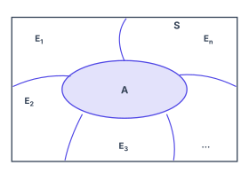
Fig 13.4 is a Venn diagram that shows the entire sample space $S$ as a large rectangle. Inside this rectangle, the space is divided by several curved lines that all radiate outward from a central region, like slices of a pie that have been pulled apart. These slices are the events $E_1, E_2, E_3, \dots, E_n$ . They are drawn so that no two slices overlap — they are mutually exclusive — and together they fill the entire rectangle — they are exhaustive. Each slice is labelled with its event name: $E_1$ sits near the top-left, $E_n$ near the top-right, $E_2$ on the left, $E_3$ at the bottom-centre, and an ellipsis ( $\dots$ ) in the bottom-right indicates that the pattern continues for any number of such events.

Across the centre of this partitioned rectangle lies a horizontal oval labelled $A$ , outlined in the same colour as the dividing curves and shaded. The key visual point is that this oval cuts through every single slice $E_i$ . Because the oval spans the whole width of the rectangle, it overlaps with each $E_i$ in a small region. Those overlapping regions are the intersections $A \cap E_1$ , $A \cap E_2$ , and so on up to $A \cap E_n$ . The figure makes it obvious that the whole of $A$ is exactly the union of all these little overlapping pieces:

A = (A \cap E_1) \cup (A \cap E_2) \cup \dots \cup (A \cap E_n).

This is the physical idea the diagram teaches: when the sample space is split into a partition — pairwise disjoint, exhaustive events with positive probabilities — any other event $A$ is automatically broken into disjoint pieces, one from each partition cell. The formula that follows from this picture is the theorem of total probability. If the events $E_1, E_2, \dots, E_n$ form a partition of $S$ , then for any event $A$ :

P(A) = P(E_1)\,P(A \mid E_1) + P(E_2)\,P(A \mid E_2) + \dots + P(E_n)\,P(A \mid E_n).

Start your 14-day free trial to unlock the full solution →

← Previous · 13.5Bayes' Theorem Next · 13.5.2 →Theorem of Total Probability