Physics · Ch 12 — Atoms

Bohr Model of the Hydrogen Atom

12.4

Bohr Model of the Hydrogen Atom

Why a New Model Was Needed

Rutherford's nuclear model — a tiny positive nucleus with electrons orbiting around it — seemed plausible at first glance. It borrowed the familiar picture of planets orbiting the Sun, with the Coulomb force replacing gravity as the central force. But this analogy breaks down in two critical ways.

First, an electron moving in a circle is constantly accelerating (centripetal acceleration). According to classical electromagnetic theory, any accelerating charged particle must radiate energy in the form of electromagnetic waves. An orbiting electron would therefore continuously lose energy, causing its orbit to shrink. The electron would spiral inward and eventually crash into the nucleus. Such an atom cannot be stable — yet atoms clearly are stable.

Second, classical theory predicts that the frequency of the emitted radiation equals the frequency of revolution. As the electron spirals inward, its angular velocity changes continuously, so the emitted light would have a continuous range of frequencies. But experiments show that hydrogen atoms emit only specific, discrete wavelengths — a line spectrum, not a continuous one.

Watch out

The Rutherford model is not wrong — it correctly describes the nuclear atom. But it is incomplete. Classical physics alone cannot explain atomic stability or the discrete spectra observed in experiments.

Bohr's Three Postulates

Niels Bohr, working in Rutherford's laboratory in 1912, accepted the nuclear model but realised that classical ideas must be modified at the atomic scale. In 1913, he proposed a theory combining classical mechanics with the new quantum ideas of Planck and Einstein. His theory rests on three postulates.

First Postulate: Stationary States

An electron in an atom can revolve in certain stable orbits without emitting radiation, contrary to classical electromagnetic theory. Each atom has a set of definite stable states, each with a fixed total energy. These are called stationary states of the atom.

Important

The first postulate directly contradicts classical electrodynamics. Bohr's radical step was to say: classical rules apply to large-scale phenomena, but at the atomic scale, new rules govern behaviour.

Second Postulate: Quantisation of Angular Momentum

The electron revolves around the nucleus only in those orbits for which its angular momentum $L$ is an integer multiple of $h/2\pi$ , where $h$ is Planck's constant ( $6.6 \times 10^{-34} \text{ J s}$ ).

L = \frac{nh}{2\pi}, \quad n = 1, 2, 3, \dots

The integer $n$ is called the principal quantum number. This condition quantises the allowed orbits — only certain discrete radii are possible.

Third Postulate: Quantum Jumps and Photon Emission

An electron can make a transition from one stationary state (energy $E_i$ ) to another of lower energy ( $E_f$ ). When it does so, a photon is emitted whose energy equals the difference between the two state energies. The frequency $\nu$ of the emitted photon is given by:

h\nu = E_i - E_f

where $E_i > E_f$ . This is the same relation Planck and Einstein used for light quanta — Bohr brought quantum ideas directly into atomic structure.

Note

The third postulate explains why atomic spectra are discrete: only specific energy differences are possible, so only specific photon frequencies (and therefore wavelengths) can be emitted.

Deriving the Radius of the $n$ th Orbit

To find the actual radii of the allowed orbits, we combine Bohr's quantisation condition with classical mechanics.

For an electron of mass $m$ and charge $-e$ moving with speed $v$ in a circular orbit of radius $r$ around a proton (charge $+e$ ), the Coulomb force provides the necessary centripetal force:

\frac{1}{4\pi\varepsilon_0} \frac{e^2}{r^2} = \frac{mv^2}{r}

From this, we get the kinetic energy:

\frac{1}{2}mv^2 = \frac{1}{8\pi\varepsilon_0} \frac{e^2}{r}

Now apply Bohr's second postulate. The angular momentum $L = mvr$ must equal $nh/2\pi$ :

mvr = \frac{nh}{2\pi}

Solving for $v$ :

v = \frac{nh}{2\pi m r}

Substitute this into the centripetal force equation:

\frac{1}{4\pi\varepsilon_0} \frac{e^2}{r^2} = \frac{m}{r} \left(\frac{nh}{2\pi m r}\right)^2

Simplify:

\frac{1}{4\pi\varepsilon_0} \frac{e^2}{r^2} = \frac{n^2 h^2}{4\pi^2 m r^3}

Multiply both sides by $r^3$ :

\frac{1}{4\pi\varepsilon_0} e^2 r = \frac{n^2 h^2}{4\pi^2 m}

Solve for $r$ :

r_n = \frac{\varepsilon_0 n^2 h^2}{\pi m e^2}

This is the radius of the $n$ th allowed orbit. For $n = 1$ (the ground state), substituting the known constants gives:

r_1 = \frac{(8.85 \times 10^{-12})(6.63 \times 10^{-34})^2}{\pi (9.11 \times 10^{-31})(1.60 \times 10^{-19})^2} \approx 5.3 \times 10^{-11} \text{ m}

This is the Bohr radius, often denoted $a_0$ . It matches the radius calculated from Rutherford scattering experiments.

Tip

The radius scales as $n^2$ : $r_n = n^2 a_0$ . The first few orbits have radii $a_0$ , $4a_0$ , $9a_0$ , $16a_0$ , and so on.

Deriving the Energy of the $n$ th State

The total energy of the electron in a stationary state is the sum of its kinetic and potential energies:

E = \frac{1}{2}mv^2 + U

The potential energy for two charges $+e$ and $-e$ separated by distance $r$ is:

U = -\frac{1}{4\pi\varepsilon_0} \frac{e^2}{r}

(The negative sign indicates an attractive force — work must be done to separate them.)

From the centripetal force equation, we already have:

\frac{1}{2}mv^2 = \frac{1}{8\pi\varepsilon_0} \frac{e^2}{r}

Therefore:

E = \frac{1}{8\pi\varepsilon_0} \frac{e^2}{r} - \frac{1}{4\pi\varepsilon_0} \frac{e^2}{r} = -\frac{1}{8\pi\varepsilon_0} \frac{e^2}{r}

Now substitute the expression for $r_n$ :

E_n = -\frac{1}{8\pi\varepsilon_0} \frac{e^2}{\left(\frac{\varepsilon_0 n^2 h^2}{\pi m e^2}\right)}

Simplify:

E_n = -\frac{1}{8\pi\varepsilon_0} \cdot \frac{\pi m e^4}{\varepsilon_0 n^2 h^2}

E_n = -\frac{m e^4}{8\varepsilon_0^2 n^2 h^2}

This is the total energy of the electron in the $n$ th stationary state of hydrogen.

Numerical Values

Substituting the known constants:

$m = 9.11 \times 10^{-31} \text{ kg}$
$e = 1.60 \times 10^{-19} \text{ C}$
$\varepsilon_0 = 8.85 \times 10^{-12} \text{ C}^2/\text{N m}^2$
$h = 6.63 \times 10^{-34} \text{ J s}$

gives:

E_n = -\frac{2.18 \times 10^{-18}}{n^2} \text{ J}

Since $1 \text{ eV} = 1.60 \times 10^{-19} \text{ J}$ , this becomes: …

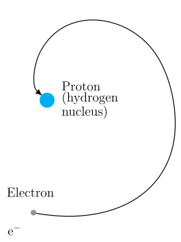
Figure 12.6An accelerated atomic electron must spiral into the nucleus as it loses energy.

Fig. 12.6 — An accelerated atomic electron must spiral into the nucleus as it loses energy.

Drawn by us to help you understand the concept clearly, and verified to make sure it's accurate. For exams, practice from your textbook's own diagram.

What Fig. 12.6 Shows

The figure is a simple schematic — not a plot with axes, but a conceptual drawing. At the centre sits a single dot labelled Proton (hydrogen nucleus). Around it, a second dot labelled Electron $e$ traces a path that is not a closed circle but a spiral that winds inward, getting closer to the nucleus with each turn. The spiral is the key visual: it shows the electron's orbit shrinking over time.

There are no axes, no gridlines, no multiple panels. The entire diagram is a before-and-after story compressed into one image — the electron starts in a large circular orbit and, as it loses energy, follows a tightening spiral until it would eventually crash into the proton.

The Physical Idea

The figure illustrates a fatal flaw in the classical (Rutherford) model of the atom. An electron moving in a circle is constantly accelerating — its velocity vector changes direction every instant. According to classical electrodynamics, any accelerating charged particle must radiate electromagnetic waves. That radiation carries away energy. As the electron loses energy, it cannot stay in the same orbit; it must move to a smaller one. Smaller orbits mean higher orbital frequency, which means faster energy loss, which means even smaller orbits — a runaway process. The inevitable end is the electron spiralling into the nucleus.

Watch out

This is not what actually happens in a real hydrogen atom. If it did, atoms would collapse in about $10^{-11}$ seconds. The fact that stable atoms exist at all was the central crisis that Bohr's model resolved.

The figure also explains a second failure of classical theory: the spectrum. If the electron's frequency changes continuously as it spirals inward, the light it emits should show a continuous spectrum — all frequencies blended together. But real hydrogen atoms emit only specific, sharp frequencies (line spectra). The spiral diagram makes this contradiction visually obvious.

The Key Formula Developed from This Figure

The textbook uses the classical picture (the spiral) to calculate the initial frequency of light that would be emitted if classical theory were correct. From Example 12.3, the electron's speed in the ground-state orbit is known:

v = 2.2 \times 10^6\ \text{m/s}

and the orbital radius is:

r = 5.3 \times 10^{-11}\ \text{m}

The orbital frequency (revolutions per second) is:

\nu = \frac{v}{2\pi r}

Substituting the numbers:

\nu = \frac{2.2 \times 10^6}{2\pi \times 5.3 \times 10^{-11}} \approx 6.6 \times 10^{15}\ \text{Hz}

Classical theory says the emitted light has exactly this frequency. So the initial frequency predicted classically is $6.6 \times 10^{15}\ \text{Hz}$ — which lies in the ultraviolet region.

Note

| Symbol | Meaning | Value (in this example) | …

Start your 14-day free trial to unlock the full solution →

← Previous · 12.3Atomic Spectra Next · 12.4 →Example 12.4 — According to the classical electromagnetic theory, calculate the initi…

Bohr Model of the Hydrogen Atom