Physics · Ch 1 — Electric Charges and Fields

Electric Flux

1.9

Electric Flux

Electric Flux: The Idea

Electric flux is a concept borrowed from fluid flow. In a fluid, the flux measures how much fluid flows through a given area per unit time. For an electric field, there is no physical flow, but we define an analogous quantity to measure the "flow" of electric field lines through a surface.

The number of electric field lines crossing a unit area placed perpendicular to the field is proportional to the field strength $E$ . Therefore, for a small planar area element of magnitude $\Delta S$ placed normal to $\vec{E}$ , the number of field lines crossing it is proportional to $E \Delta S$ .

Dependence on Orientation

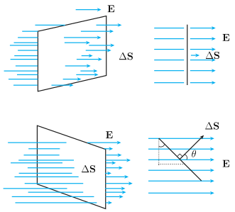
If the area element is tilted by an angle $\theta$ relative to the field direction, the effective area presented to the field is the projection of the area onto a plane perpendicular to $\vec{E}$ . This projected area is $\Delta S \cos \theta$ .

When $\theta = 0^\circ$ (area normal to field), the flux is maximum.
When $\theta = 90^\circ$ (area parallel to field), no field lines cross it, so flux is zero.

Thus, the number of field lines crossing the area is proportional to $E \Delta S \cos \theta$ .

Area as a Vector

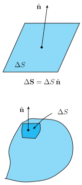
Because orientation matters, an area element must be treated as a vector $\Delta \vec{S}$ . Its magnitude is $\Delta S$ , and its direction is along the normal to the plane.

For a closed surface, the convention is that the normal points outward (out of the volume enclosed). The area vector is then $\Delta \vec{S} = \Delta S \, \hat{n}$ , where $\hat{n}$ is the outward unit normal.

Definition of Electric Flux

The electric flux $\Delta \phi$ through a small area element $\Delta \vec{S}$ is defined as the dot product of the electric field $\vec{E}$ and the area vector $\Delta \vec{S}$ :

\Delta \phi = \vec{E} \cdot \Delta \vec{S} = E \, \Delta S \cos \theta

$\vec{E}$ : electric field at the location of the area element.
$\Delta \vec{S}$ : area vector (magnitude $\Delta S$ , direction along outward normal $\hat{n}$ ).
$\theta$ : angle between $\vec{E}$ and the outward normal $\hat{n}$ .

This expression can be interpreted in two equivalent ways:

$E (\Delta S \cos \theta)$ : the field strength times the projected area perpendicular to $\vec{E}$ .
$(E \cos \theta) \Delta S$ : the component of $\vec{E}$ along the normal times the area magnitude. …

Figure 1.15Dependence of flux on the inclination q between E and n̂.

Fig. 1.15 — Dependence of flux on the inclination q between E and n̂.

Drawn by us to help you understand the concept clearly, and verified to make sure it's accurate. For exams, practice from your textbook's own diagram.

What the Figure Shows

The figure consists of four small panels, each illustrating a uniform horizontal electric field $\mathbf{E}$ (represented by evenly spaced parallel lines) and a small planar area element $\Delta S$ . The area element is drawn as a short line segment (its edge-on view) with its associated area vector $\Delta \mathbf{S}$ (a normal arrow) sticking out perpendicular to it. A dotted helper line shows the direction of $\mathbf{E}$ for comparison.

Top-left panel: The area element is held face-on to the field — its normal $\hat{\mathbf{n}}$ is exactly parallel to $\mathbf{E}$ ( $\theta = 0^\circ$ ). All field lines cross the element, so the flux is maximum.
Top-right panel: The area element is edge-on to the field, with its area vector $\Delta \mathbf{S}$ pointing along $\mathbf{E}$ (again $\theta = 0^\circ$ ). This is the same orientation as the top-left panel, just drawn from a different perspective — the element is still perpendicular to the field.
Bottom-left panel: The element is tilted at some angle $\theta$ relative to $\mathbf{E}$ . Fewer field lines cross it because the effective area presented to the field is smaller.
Bottom-right panel: The element is again edge-on, but now its normal $\hat{\mathbf{n}}$ makes an angle $\theta$ with $\mathbf{E}$ . A right-angle mark is drawn between $\Delta \mathbf{S}$ and the element itself, emphasizing that the area vector is always perpendicular to the surface.

Physical Idea

The figure teaches that electric flux depends not only on the strength of the field and the size of the area, but also on the orientation of the area relative to the field. When the area is perpendicular to $\mathbf{E}$ , all field lines pass through it — flux is maximum. When it is tilted, only the component of the area perpendicular to $\mathbf{E}$ (the projected area $\Delta S \cos\theta$ ) is effective. When the area is parallel to $\mathbf{E}$ ( $\theta = 90^\circ$ ), no field lines cross it — flux is zero. This is why area must be treated as a vector: its direction (the normal) determines how much of the field actually "flows" through it.

Key Formula

The textbook defines electric flux $\Delta \Phi$ through a small area element $\Delta \mathbf{S}$ as:

\Delta \Phi = \mathbf{E} \cdot \Delta \mathbf{S} = E \, \Delta S \cos\theta

where:

$\mathbf{E}$ is the electric field vector (uniform over the element), …

Figure 1.16Convention for defining normal n̂ and DS.

Fig. 1.16 — Convention for defining normal n̂ and DS.

Drawn by us to help you understand the concept clearly, and verified to make sure it's accurate. For exams, practice from your textbook's own diagram.

What the Figure Shows

The figure consists of two separate drawings that together establish the area vector convention used throughout electrostatics.

Top drawing: A small, flat surface element labelled $\Delta S$ (the magnitude of the area). A unit vector $\hat{n}$ is drawn emerging from the centre of this element, nearly vertical. Below the element, the relation $\Delta \mathbf{S} = \Delta S \, \hat{n}$ is written. This drawing shows that any planar area can be treated as a vector — its magnitude is the area $\Delta S$ , and its direction is along the normal $\hat{n}$ to the plane.

Bottom drawing: An irregular closed surface (like a potato shape). On its upper-left boundary, a small patch is highlighted. From this patch, an arrow labelled $\hat{n}$ points outward — away from the interior of the closed surface. Next to the patch, the label $\Delta \mathbf{S}$ appears, connected by a leader line. This drawing shows the convention for closed surfaces: the area vector $\Delta \mathbf{S}$ for every small element is taken along the outward normal.

The Physical Idea

The figure teaches two essential ideas:

Area as a vector — The orientation of a surface matters when calculating flux. Tilting the surface changes how much of the field "flows" through it. The vector $\Delta \mathbf{S}$ captures both the size and the orientation.
Outward normal convention — For a closed surface, there is an ambiguity: the normal can point inward or outward. The figure fixes this by choosing the outward normal as the direction of $\Delta \mathbf{S}$ . This convention is crucial for Gauss's law, where the total flux through a closed surface depends on the net charge enclosed.

Key Formula Developed with This Figure

The textbook uses this figure to define electric flux through a small area element:

\Delta \Phi = \mathbf{E} \cdot \Delta \mathbf{S} = E \, \Delta S \cos \theta

where:

$\Delta \Phi$ = electric flux through the area element (in $\text{N C}^{-1} \text{m}^2$ )
$\mathbf{E}$ = electric field vector at the location of the element …

Start your 14-day free trial to unlock the full solution →

← Previous · 1.8Electric Field Lines Next · 1.10 →Electric Dipole