Physics · Ch 14 — Waves

Standing Waves and Normal Modes

14.6.1

Standing Waves and Normal Modes

When a wave reflects from two boundaries — as in a string fixed at both ends or an air column in a pipe — the repeated reflections eventually produce a steady, non-moving wave pattern. These patterns are called standing waves or stationary waves.

Mathematical Description of Standing Waves

Consider a wave travelling along the positive x-direction and another wave of the same amplitude and wavelength travelling in the negative x-direction. Taking the phase constant $\phi = 0$ , we write:

y_1(x, t) = a \sin(kx - \omega t)

y_2(x, t) = a \sin(kx + \omega t)

By the principle of superposition, the resultant displacement is:

y(x, t) = y_1(x, t) + y_2(x, t) = a[\sin(kx - \omega t) + \sin(kx + \omega t)]

Using the trigonometric identity $\sin(A+B) + \sin(A-B) = 2\sin A \cos B$ , we obtain:

y(x, t) = 2a \sin(kx) \cos(\omega t)

This is the equation of a standing wave.

Important

In a standing wave, the terms $kx$ and $\omega t$ appear separately — not in the combination $kx - \omega t$ as in a travelling wave. The amplitude $2a \sin(kx)$ varies from point to point, but every element of the string oscillates with the same angular frequency $\omega$ and the same phase.

Key Features of Standing Waves

The amplitude at any position $x$ is $|2a \sin(kx)|$ . This means:

Nodes: Points where the amplitude is zero — $\sin(kx) = 0$ . These points never move.
Antinodes: Points where the amplitude is maximum — $|\sin(kx)| = 1$ . These points oscillate with the largest amplitude.

The wave pattern does not travel to the right or left; it simply oscillates in place. Hence the name "standing" or "stationary" wave.

Positions of Nodes and Antinodes

Nodes occur when $\sin(kx) = 0$ , which gives:

kx = n\pi, \quad n = 0, 1, 2, 3, \dots

Since $k = \frac{2\pi}{\lambda}$ , we get:

x = n\frac{\lambda}{2}, \quad n = 0, 1, 2, 3, \dots

The distance between any two successive nodes is $\frac{\lambda}{2}$ .

Antinodes occur when $|\sin(kx)| = 1$ , which gives:

kx = \left(n + \frac{1}{2}\right)\pi, \quad n = 0, 1, 2, 3, \dots

With $k = \frac{2\pi}{\lambda}$ , we get:

x = \left(n + \frac{1}{2}\right)\frac{\lambda}{2}, \quad n = 0, 1, 2, 3, \dots

The distance between any two successive antinodes is also $\frac{\lambda}{2}$ .

Note

A node and the next antinode are separated by $\frac{\lambda}{4}$ .

Normal Modes of a String Fixed at Both Ends

Consider a stretched string of length $L$ fixed at both ends. Taking one end at $x = 0$ , the boundary conditions are that $x = 0$ and $x = L$ must be nodes.

The condition at $x = 0$ is automatically satisfied by $\sin(0) = 0$ . For $x = L$ to be a node, we require:

\sin(kL) = 0 \quad \Rightarrow \quad kL = n\pi, \quad n = 1, 2, 3, \dots

Since $k = \frac{2\pi}{\lambda}$ , this gives:

L = n\frac{\lambda}{2}, \quad n = 1, 2, 3, \dots

Thus the possible wavelengths are:

\lambda_n = \frac{2L}{n}, \quad n = 1, 2, 3, \dots

The corresponding frequencies, using $v = \nu\lambda$ , are:

\nu_n = \frac{nv}{2L}, \quad n = 1, 2, 3, \dots

These are the natural frequencies or normal modes of oscillation of the system.

Important

|------|-----|----------------------|-------------------|------|

| Fundamental | 1 | $2L$ | $\frac{v}{2L}$ | First harmonic |

| Second | 2 | $L$ | $\frac{v}{L}$ | Second harmonic |

| Third | 3 | $\frac{2L}{3}$ | $\frac{3v}{2L}$ | Third harmonic |

| $n$ th | $n$ | $\frac{2L}{n}$ | $\frac{nv}{2L}$ | $n$ th harmonic |

The fundamental frequency ( $n=1$ ) is the lowest possible natural frequency. All higher frequencies are integer multiples of the fundamental — hence the term "harmonics."

Watch out

A string does not have to vibrate in just one mode. Its actual vibration is generally a superposition of several modes. Which modes are prominent depends on where the string is plucked or bowed — this is the principle behind musical instruments like the sitar and violin.

Normal Modes of an Air Column with One End Closed

Consider a pipe of length $L$ with one end closed and the other open. The closed end (in contact with water, for example) is a node — here pressure changes are largest but displacement is zero. The open end is an antinode — here pressure changes are smallest and displacement amplitude is maximum.

Take the closed end at $x = 0$ (node condition already satisfied). For the open end at $x = L$ to be an antinode:

L = \left(n + \frac{1}{2}\right)\frac{\lambda}{2}, \quad n = 0, 1, 2, 3, \dots

The possible wavelengths are:

\lambda_n = \frac{2L}{\left(n + \frac{1}{2}\right)} = \frac{4L}{2n+1}, \quad n = 0, 1, 2, 3, \dots

The corresponding natural frequencies are:

\nu_n = \left(n + \frac{1}{2}\right)\frac{v}{2L} = \frac{(2n+1)v}{4L}, \quad n = 0, 1, 2, 3, \dots

Important

For a pipe closed at one end, only odd harmonics are present. The fundamental frequency ( $n=0$ ) is $\frac{v}{4L}$ . The higher frequencies are $3\frac{v}{4L}$ , $5\frac{v}{4L}$ , and so on — odd multiples of the fundamental.

Normal Modes of an Air Column Open at Both Ends

For a pipe open at both ends, each end is an antinode. The analysis shows that such a pipe generates all harmonics — both even and odd.

Tip

The pattern is: open-open pipe → all harmonics; closed-open pipe → only odd harmonics. This difference arises because the boundary conditions at the two ends are the same for an open-open pipe (both antinodes) but different for a closed-open pipe (one node, one antinode).

Resonance

When an external driving frequency matches one of the natural frequencies of a system, resonance occurs — the system vibrates with large amplitude. This applies to both strings and air columns. …

Figure 14.12Stationary waves arising from superposition of two harmonic waves travelling in opposite directions. The nodes remain fixed at all times.

Fig. 14.12 — Stationary waves arising from superposition of two harmonic waves travelling in opposite directions. The nodes remain fixed at all times.

Drawn by us to help you understand the concept clearly, and verified to make sure it's accurate. For exams, practice from your textbook's own diagram.

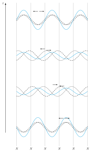
The figure shows a vertical time axis on the left, with four horizontal rows stacked one above the other. Each row represents a different instant of time, increasing upward. In every row, three curves are drawn across the page: a right‑moving wave (say, red), a left‑moving wave (say, green), and their superposition — the resultant standing wave — shown in blue. Vertical dashed lines run from top to bottom of the figure, marking fixed positions called nodes, labelled N at the bottom. The nodes are the points where the blue resultant wave is always zero, regardless of which time row you look at.

The horizontal axis is position ( $x$ ) along the string. The vertical displacement of each wave at that position is plotted as a curve. The right‑moving wave travels to the right as time increases; the left‑moving wave travels to the left. Because they have the same amplitude, frequency, and speed, their superposition produces a stationary pattern — the standing wave — whose shape oscillates in place but whose nodes never move.

The physical idea is that when two identical harmonic waves travel in opposite directions, they interfere. At certain points (nodes), the two waves always cancel exactly, so the resultant displacement is permanently zero. At other points (antinodes), the waves add constructively, giving maximum displacement that varies with time. The figure shows this clearly: the blue standing wave changes shape from row to row (it goes flat, then bulges upward, then flat again, then bulges downward), but the dashed node lines remain fixed.

The textbook develops the mathematics of this superposition. If the right‑moving wave is $y_1(x,t) = A \sin(kx - \omega t)$ and the left‑moving wave is $y_2(x,t) = A \sin(kx + \omega t)$ , their sum gives the standing wave:

y(x,t) = y_1 + y_2 = 2A \sin(kx) \cos(\omega t)

Here $A$ is the amplitude of each individual travelling wave, $k = 2\pi/\lambda$ is the wave number ( $\lambda$ is the wavelength), and $\omega = 2\pi f$ is the angular frequency ( $f$ is the frequency). The factor $\sin(kx)$ describes the spatial shape — it is zero at positions where $kx = n\pi$ , i.e. $x = n\lambda/2$ for integer $n$ . Those are the nodes. The factor $\cos(\omega t)$ tells how the entire pattern oscillates in time: at $t=0$ the displacement is maximum, at a quarter period later it is zero everywhere, and so on. …

Figure 14.13The first six harmonics of vibrations of a stretched string fixed at both ends.

Fig. 14.13 — The first six harmonics of vibrations of a stretched string fixed at both ends.

Drawn by us to help you understand the concept clearly, and verified to make sure it's accurate. For exams, practice from your textbook's own diagram.

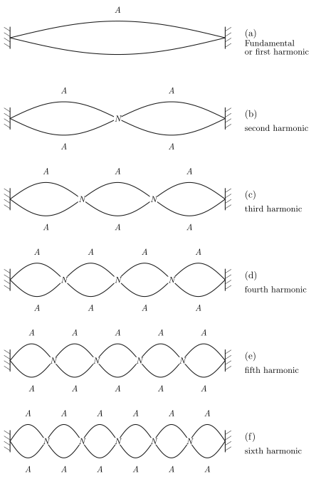
The figure shows six separate panels, labelled (a) through (f), stacked vertically. Each panel is a snapshot of a stretched string clamped at both ends — the clamps are drawn as hatched blocks on the left and right. The string itself is shown as a horizontal line when it is at rest, and as a smooth curve when it is vibrating.

In each panel, the string is displaced into a standing wave pattern. The number of loops (the bulging segments between successive nodes) increases from one in panel (a) to six in panel (f). Nodes are marked with the letter N — these are the points that never move. Antinodes are marked with the letter A — these are the points of maximum displacement. The clamps themselves are always nodes because the string cannot move there.

The horizontal axis represents position along the string from one fixed end to the other. The vertical axis represents the instantaneous displacement of the string from its equilibrium position. Because the figure shows a snapshot, the string appears frozen at one instant; in reality, each loop would be oscillating up and down, with the antinode moving between its maximum positive and maximum negative displacement.

Note

The figure does not show the string moving — it shows the shape of the standing wave at the moment of maximum displacement. At other times the amplitude is smaller, but the positions of nodes and antinodes remain fixed.

The physical idea is that a string fixed at both ends can only vibrate in certain specific patterns, called normal modes or harmonics. Each mode has a characteristic number of loops and a characteristic frequency. The first harmonic (fundamental) has one loop, the second harmonic has two loops, and so on. The figure makes this progression visually clear: as the harmonic number increases, the string is divided into more and more vibrating segments, and the wavelength becomes shorter.

The key formula that the textbook develops from this figure is the relationship between the length of the string $L$ , the wavelength $\lambda_n$ of the $n$ th harmonic, and the harmonic number $n$ :

\lambda_n = \frac{2L}{n}, \quad n = 1, 2, 3, \dots

Here $L$ is the distance between the two fixed ends (the length of the string), $n$ is the harmonic number (also called the mode number), and $\lambda_n$ is the wavelength of the standing wave for that harmonic. For the fundamental ( $n=1$ ), the wavelength is $2L$ — the string holds exactly half a wavelength. For the second harmonic ( $n=2$ ), the wavelength is $L$ — the string holds one full wavelength. For the third harmonic ( $n=3$ ), $\lambda_3 = 2L/3$ , and so on.

The frequency of each harmonic follows from the wave speed $v$ on the string:

f_n = \frac{v}{\lambda_n} = \frac{nv}{2L}, \quad n = 1, 2, 3, \dots

So the frequencies are integer multiples of the fundamental frequency $f_1 = v/(2L)$ . This is why the set of modes is called the harmonic series. …

Figure 14.14Normal modes of an air column open at one end and closed at the other. Only odd harmonics are possible.

Fig. 14.14 — Normal modes of an air column open at one end and closed at the other. Only odd harmonics are possible.

Drawn by us to help you understand the concept clearly, and verified to make sure it's accurate. For exams, practice from your textbook's own diagram.

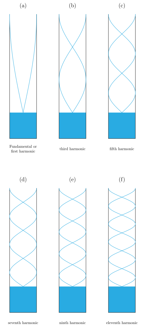
The figure shows six vertical glass tubes, each closed at the bottom by a water surface and open at the top. The water surface acts as a rigid boundary — a node (point of zero displacement) for the air column. The open top is a free boundary — an antinode (point of maximum displacement). Inside each tube, the figure draws the standing-wave envelope: the shape of the air column's displacement at an instant, for the first six allowed modes.

The tubes are labelled (a) through (f). Tube (a) shows the fundamental mode (first harmonic): the air column has a node at the water surface and an antinode at the open top — that is one-quarter of a wavelength. Tube (b) shows the third harmonic: the envelope has one full node at the water surface, one node inside the column, and an antinode at the top — three-quarters of a wavelength. Tube (c) shows the fifth harmonic (five-quarters of a wavelength), and so on up to tube (f) which shows the eleventh harmonic (eleven-quarters of a wavelength).

The key physical idea is that only odd harmonics are possible in a pipe closed at one end. The water surface forces a node; the open top forces an antinode. The distance between a node and the nearest antinode is always $\lambda/4$ . For the $n$ th allowed mode, the length $L$ of the air column must satisfy:

L = (2n-1)\frac{\lambda_n}{4}, \quad n = 1,2,3,\dots

where $n=1$ gives the fundamental, $n=2$ the third harmonic, $n=3$ the fifth, and so on. The corresponding frequencies are:

f_n = \frac{v}{\lambda_n} = (2n-1)\frac{v}{4L} = (2n-1)f_1

where $v$ is the speed of sound in air and $f_1 = v/4L$ is the fundamental frequency. …

Start your 14-day free trial to unlock the full solution →

← Previous · 14.6Reflection of Waves Next · 14.6.1 →Example 14.5 — A pipe, 30.0cm long, is open at both ends. Which harmonic mode of the …