Economics · Ch 9 — Production and Costs

Production Function

9.1

Production Function

3.1 Production Function

A production function is the technical relationship that connects the inputs a firm uses to the output it produces. For any given combination of inputs, the production function tells us the maximum quantity of output that can be obtained. This is not just any output level — it is the highest possible output from those inputs, assuming the firm operates efficiently.

Consider a farmer growing wheat. To keep things simple, suppose he uses only two inputs: land and labour. The production function tells him the maximum wheat he can grow with, say, 1 hectare of land and 2 hours of labour per day. If that combination yields 2 tonnes of wheat, the production function captures that exact relation.

One possible form such a function could take is:

q = K \times L

where:

$q$ = quantity of wheat produced (in tonnes)
$K$ = area of land used (in hectares)
$L$ = labour hours per day

This simple equation shows that if either $K$ or $L$ increases, $q$ also increases. For any specific pair of $K$ and $L$ , there is exactly one value of $q$ .

Important

A production function always gives the maximum output possible from a given set of inputs. This means it deals only with efficient production — it is not possible to get more output from the same inputs. If you could, the original function was not a true production function.

The production function is defined for a given technology. Technology here means the body of knowledge and techniques available for production. If technology improves — say, a better seed variety or a more efficient plough — the same inputs can produce more output. That would be a new production function.

Factors of Production

The inputs a firm uses are called factors of production. In reality, a firm may use many inputs — land, labour, capital, raw materials, energy, and so on. However, for the purpose of this chapter, we consider a firm that uses only two factors: labour ( $L$ ) and capital ( $K$ ).

We write the production function as:

q = f(L, K) \qquad(3.1)

This is a general form. It says that output $q$ is some function $f$ of labour $L$ and capital $K$ . The exact mathematical form of $f$ depends on the technology.

A Numerical Example: Table 3.1

The textbook provides a concrete numerical production function in Table 3.1. The table shows output levels for different combinations of labour and capital.

				Capital
	0	1	2	3	4	5	6
Labour
0	0	0	0	0	0	0	0
1	0	1	3	7	10	12	13
2	0	3	10	18	24	29	33
3	0	7	18	30	40	46	50
4	0	10	24	40	50	56	57
5	0	12	29	46	56	58	59
6	0	13	33	50	57	59	60

Reading this table:

The left column shows units of labour.
The top row shows units of capital.
Each cell gives the maximum output for that combination of labour and capital.

For example:

With 1 unit of labour and 1 unit of capital, output is 1 unit.
With 2 units of labour and 2 units of capital, output is 10 units.
With 3 units of labour and 2 units of capital, output is 18 units.

Note

Notice that when either input is zero, output is zero. Both labour and capital are necessary for production in this example. As you move right along any row (increasing capital) or down any column (increasing labour), output increases. This is the typical pattern: more inputs yield more output.

Key Observations from the Table

Several important features stand out:

Both inputs are essential. If labour is zero, output is zero regardless of how much capital is used. Similarly, if capital is zero, output is zero regardless of labour. This reflects the fact that production requires both factors working together.
Output increases with each input. As you increase labour (moving down a column), output rises. As you increase capital (moving right along a row), output also rises. This is the property of positive marginal products — each additional unit of an input adds to total output.
The relationship is not linear. Notice that doubling both inputs does not always double output. For instance, going from (1 labour, 1 capital) to (2 labour, 2 capital) increases output from 1 to 10 — a tenfold increase. But going from (2 labour, 2 capital) to (4 labour, 4 capital) increases output from 10 to 50 — only a fivefold increase. This pattern of changing returns will be explored in later sections.
The table represents a specific technology. If technology improved, the numbers in the table would change — for the same inputs, output would be higher.

Watch out

Do not confuse the production function with a cost function. The production function is purely a physical relationship between inputs and output, measured in units like tonnes of wheat or number of chairs. It does not involve prices or money. Costs come later, when we multiply input quantities by their prices.

Isoquants

Note

Isoquant

In Chapter 2 we studied indifference curves. An isoquant is the analogous idea for production — just an alternative way of representing the production function. An isoquant is the set of all combinations of the two inputs that yield the same maximum level of output, and each isoquant is labelled with the output level it represents.

Look again at Table 3.1. An output of 10 units can be produced in three ways — $(L=4, K=1)$ , $(L=2, K=2)$ and $(L=1, K=4)$ . All three input combinations lie on the same isoquant, the one representing an output of 10.

…

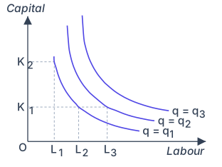
Isoquants for three output levels q1, q2 and q3 — each downward-sloping curve shows all the combinations of labour (L) and capital (K) that give the same maximum output, with higher isoquants (further from the origin) representing higher output levels

Drawn by us to help you understand the concept clearly, and verified to make sure it's accurate. For exams, practice from your textbook's own diagram.

An isoquant is the set of all input combinations that yield the same maximum possible output, so it works like an indifference curve for production. The combinations $(L_1, K_2)$ and $(L_2, K_1)$ both lie on the isoquant $q = q_1$ , meaning both produce exactly the same output. Keeping capital fixed at $K_1$ and raising labour to $L_3$ lifts the firm to the higher isoquant $q = q_2$ — with positive marginal products, more of one input (the other …

Start your 14-day free trial to unlock the full solution →

← Previous · introIntroduction Next · 9.2 →The Short Run and the Long Run