Chemistry · Ch 3 — Chemical Kinetics

Rate of a Chemical Reaction

3.1

Rate of a Chemical Reaction

What Do We Mean by the "Rate" of a Reaction?

Different reactions proceed at very different speeds. Ionic reactions, such as the precipitation of silver chloride when solutions of silver nitrate and sodium chloride are mixed, are essentially instantaneous. Rusting of iron in moist air, by contrast, is extremely slow. Processes such as the inversion of cane sugar or the hydrolysis of starch fall somewhere in between, proceeding at a moderate pace.

Just as the speed of a moving object is described as the change in its position over a time interval, the rate of a chemical reaction is described as the change in the concentration of a reactant or a product over a unit of time. A rate can be stated in two equivalent ways:

as the rate at which the concentration of any one reactant is decreasing, or
as the rate at which the concentration of any one product is increasing.

Kinetic studies of this kind matter because they let us pin down not just how fast a reaction runs but also which conditions — concentration, temperature, pressure, and the presence of a catalyst — change that speed.

Setting Up the Rate Expression

Consider a simple hypothetical reaction, with the volume of the system held constant:

R \rightarrow P

Suppose $[\mathrm{R}]_1$ and $[\mathrm{P}]_1$ are the concentrations of R and P at time $t_1$ , and $[\mathrm{R}]_2$ , $[\mathrm{P}]_2$ are their concentrations at a later time $t_2$ . Then

\Delta t = t_2 - t_1, \qquad \Delta[\mathrm{R}] = [\mathrm{R}]_2 - [\mathrm{R}]_1, \qquad \Delta[\mathrm{P}] = [\mathrm{P}]_2 - [\mathrm{P}]_1

(square brackets denote molar concentration). Because R is being consumed, $\Delta[\mathrm{R}]$ works out to a negative number, while $\Delta[\mathrm{P}]$ is positive since P is being formed.

Using these, the rate can be written either as the rate of disappearance of the reactant or the rate of appearance of the product:

\text{Rate of disappearance of R} = \frac{\text{Decrease in concentration of R}}{\text{Time taken}} = -\frac{\Delta[\mathrm{R}]}{\Delta t}

\text{Rate of appearance of P} = \frac{\text{Increase in concentration of P}}{\text{Time taken}} = +\frac{\Delta[\mathrm{P}]}{\Delta t}

Note

The minus sign in front of $\Delta[\mathrm{R}]/\Delta t$ is not arbitrary — it simply cancels the fact that $\Delta[\mathrm{R}]$ itself is negative, so that the rate of the reaction comes out as a positive quantity regardless of whether it is tracked through a reactant or a product.

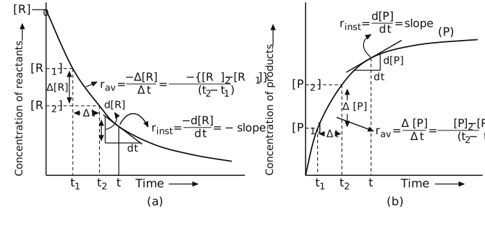
These two expressions describe the average rate of a reaction, denoted $r_{av}$ . As the name suggests, it is an average taken over the chosen interval — its value depends jointly on how much the concentration changed and how long that change took.

Figure 3.1Instantaneous and average rate of a reaction

Fig. 3.1 — Instantaneous and average rate of a reaction

Drawn by us to help you understand the concept clearly, and verified to make sure it's accurate. For exams, practice from your textbook's own diagram.

The figure presents two side-by-side concentration–time graphs that together illustrate the two complementary ways to quantify how fast a reaction proceeds.

What each panel shows

Panel (a): The vertical axis is labelled concentration of reactant, $[R]$ $[R]$ , and the horizontal axis is time, $t$ $t$ . The curve starts at the initial concentration $[R]_0$ $[R]_{0}$ and falls smoothly as the reactant is consumed.
- Dotted construction lines mark the concentrations $[R_1]$ and $[R_2]$ at times $t_1$ and $t_2$ , and the annotated ratio of those changes gives the average rate over that interval:

\text{average rate} = -\frac{\Delta [R]}{\Delta t}

where $\Delta [R] = [R]_{t_2} - [R]_{t_1}$ is negative (concentration decreases), so the minus sign makes the rate positive.

A tangent line touches the curve at a single time $t$ . Its slope gives the instantaneous rate at that moment:

\text{instantaneous rate} = -\frac{d[R]}{dt}

Panel (b): The vertical axis is concentration of product, $[P]$ $[P]$ , and the horizontal axis is again time, $t$ $t$ . The curve rises from zero as product forms.
- The same dotted-construction reading between $t_1$ and $t_2$ gives the average rate:

\text{average rate} = +\frac{\Delta [P]}{\Delta t}

(no minus sign because $\Delta [P]$ is positive).

The tangent at time $t$ gives the instantaneous rate:

\text{instantaneous rate} = +\frac{d[P]}{dt}

The physical idea

The figure teaches that the rate of a reaction is not constant — it changes as reactants are used up. The average rate is a coarse measure over a finite time interval, useful for comparing different intervals (as in Table 3.1 of the textbook). The instantaneous rate is the true rate at a specific instant, obtained by shrinking the time interval to zero. Both rates are defined as positive quantities by convention: for reactants we add a minus sign because $[R]$ decreases; for products we use the positive change directly.

Key formulas developed from the figure

The textbook uses the figure to introduce the fundamental definitions:

Average rate (over a time interval $\Delta t$ ):

r_{\text{av}} = -\frac{\Delta [R]}{\Delta t} = +\frac{\Delta [P]}{\Delta t}

Instantaneous rate (at a particular time $t$ ): …

From Average Rate to Instantaneous Rate

Because an average rate is computed over a finite stretch of time, it stays the same number for that whole stretch and so cannot tell us the rate at one particular moment. Example 3.1 illustrates this directly: it walks through the hydrolysis of butyl chloride,

\mathrm{C_4H_9Cl + H_2O \rightarrow C_4H_9OH + HCl}

tabulating the average rate over a series of successive time intervals (see the accompanying data table for this reaction) — and that computed rate is clearly seen to fall steadily as the reaction proceeds and the reactant is used up.

Table 3.1Average rates of hydrolysis of butyl chloride

$[C_4H_9Cl]_{t_1}$ /mol L⁻¹	$[C_4H_9Cl]_{t_2}$ /mol L⁻¹	$t_1$ /s	$t_2$ /s	$r_{av}\times10^{4}$ /mol L⁻¹ s⁻¹
0.100	0.0905	0	50	1.90
0.0905	0.0820	50	100	1.70
0.0820	0.0741	100	150	1.58
0.0741	0.0671	150	200	1.40
0.0671	0.0549	200	300	1.22
0.0549	0.0439	300	400	1.10
0.0439	0.0335	400	500	1.04
0.0210	0.017	700	800	0.4

To describe the rate at a single instant rather than over an interval, we shrink the time interval down until it becomes infinitesimally small, $\mathrm{d}t$ (that is, we let $\Delta t \to 0$ ). This gives the instantaneous rate:

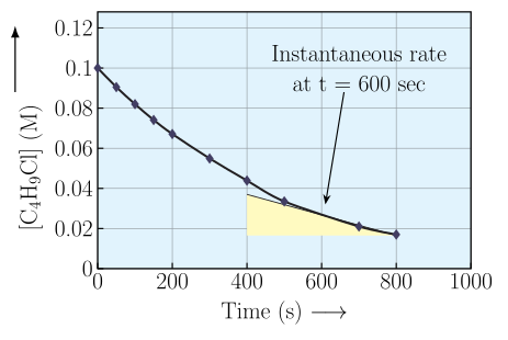
r_{av} = \frac{-\Delta[\mathrm{R}]}{\Delta t} = \frac{\Delta[\mathrm{P}]}{\Delta t}

\text{as } \Delta t \to 0, \qquad r_{inst} = \frac{-\mathrm{d}[\mathrm{R}]}{\mathrm{d}t} = \frac{\mathrm{d}[\mathrm{P}]}{\mathrm{d}t}

Graphically, the instantaneous rate at a given time $t$ is obtained by plotting concentration against time and drawing a tangent to the curve at that point — the slope of this tangent is the instantaneous rate (illustrated for a general reactant/product pair in the accompanying concentration-vs-time figure, and worked through concretely for the butyl-chloride hydrolysis data, where a tangent is drawn on the concentration curve at a chosen instant and its slope read off as the rate at that moment

Figure 3.2Instantaneous rate of hydrolysis of butyl chloride (C4H9Cl)

Fig. 3.2 — Instantaneous rate of hydrolysis of butyl chloride (C4H9Cl)

Drawn by us to help you understand the concept clearly, and verified to make sure it's accurate. For exams, practice from your textbook's own diagram.

What the Figure Shows

The figure is a concentration–time graph for the hydrolysis of butyl chloride ( $\text{C}_4\text{H}_9\text{Cl}$ ).

Y‑axis: $[\text{C}_4\text{H}_9\text{Cl}]$ in mol L⁻¹, ranging from 0 to 0.12.
X‑axis: Time in seconds, from 0 to 1000.

A smooth, falling curve passes through the data points from Table 3.1 (e.g., at $t=0$ , $[\text{C}_4\text{H}_9\text{Cl}] = 0.100$ mol L⁻¹; at $t=800$ s, $0.017$ mol L⁻¹).

At $t = 600$ s, a straight tangent line is drawn touching the curve. The tangent is labelled “Instantaneous rate at $t = 600$ sec”.

The slope of this tangent (change in concentration divided by change in time) gives the instantaneous rate at that exact moment.

Physical Idea Taught

The graph shows that the rate of a reaction is not constant — it decreases as the reactant is used up.

The average rate over a time interval is the slope of the chord between two points on the curve.
The instantaneous rate at a specific time is the slope of the tangent to the curve at that time.

This distinction is crucial: average rate hides the variation within the interval, while instantaneous rate captures the true speed at a single instant.

Key Formula Developed with This Figure

The textbook defines instantaneous rate mathematically as:

r_{\text{inst}} = -\frac{d[\text{R}]}{dt}

where:

$[\text{R}]$ = concentration of reactant (here, $\text{C}_4\text{H}_9\text{Cl}$ ) in mol L⁻¹
$t$ = time in seconds
The negative sign makes the rate positive because $d[\text{R}]$ is negative (reactant concentration decreases). …

Reading the tangent drawn at $t = 600$ s off this plot gives the instantaneous rate directly from its slope:

r_{inst} = -\frac{0.0165 - 0.037}{(800 - 400)\text{ s}} \text{ mol L}^{-1} = 5.12 \times 10^{-5} \text{ mol L}^{-1}\text{s}^{-1}

Tangents drawn at other instants give a falling sequence of instantaneous rates: $1.22 \times 10^{-4}$ mol L $^{-1}$ s $^{-1}$ at $t = 250$ s, $1.0 \times 10^{-4}$ at $t = 350$ s, and $6.4 \times 10^{-5}$ at $t = 450$ s — the rate keeps falling as the reactant is used up.

Units of Rate of a Reaction

Since rate is a change in concentration divided by a change in time, its units are always concentration ÷ time. When concentration is expressed in $\mathrm{mol\ L^{-1}}$ and time in seconds, the rate comes out in

\mathrm{mol\ L^{-1}\,s^{-1}}

For a reaction involving gases, it is often more convenient to track partial pressures instead of molar concentrations. Since, at constant temperature, the concentration of a gas is directly proportional to its partial pressure, the rate can equally well be expressed as the rate of change of partial pressure of a reactant or product, in which case the units become

\mathrm{atm\ s^{-1}}

Building in the Stoichiometric Coefficients

The expressions above work cleanly when every species in the reaction has a coefficient of one, as in

\mathrm{Hg(l) + Cl_2(g) \rightarrow HgCl_2(s)}

Here the rate of disappearance of either reactant equals the rate of appearance of the product:

\text{Rate} = -\frac{\Delta[\mathrm{Hg}]}{\Delta t} = -\frac{\Delta[\mathrm{Cl_2}]}{\Delta t} = \frac{\Delta[\mathrm{HgCl_2}]}{\Delta t}

But once the coefficients differ from one, the raw rates of change of the different species are no longer numerically equal to each other, even though they describe the same reaction. Take the decomposition

\mathrm{2HI(g) \rightarrow H_2(g) + I_2(g)}

Two moles of HI disappear for every one mole each of $\mathrm{H_2}$ and $\mathrm{I_2}$ formed, so the rate of consumption of HI is twice the rate of formation of either product. To make the numbers agree, $\Delta[\mathrm{HI}]/\Delta t$ is divided by its coefficient, 2:

\text{Rate} = -\frac{1}{2}\frac{\Delta[\mathrm{HI}]}{\Delta t} = \frac{\Delta[\mathrm{H_2}]}{\Delta t} = \frac{\Delta[\mathrm{I_2}]}{\Delta t}

The same idea extends to any reaction, however many species and however large the coefficients, as in …

Start your 14-day free trial to unlock the full solution →

← Previous · introIntroduction Next · 3.1 →Example 3.1 — From the concentrations of C₄H₉Cl (butyl chloride) at different times …