Mathematics · Ch 2 — Inverse Trigonometric Functions
Basic Concepts
Basic Concepts
2.2 Basic Concepts — Inverse Trigonometric Functions
From Functions to Inverse Functions
In Class XI the six trigonometric functions were studied as mappings on subsets of , each with a specific domain and range:
- Sine:
- Cosine:
- Tangent:
- Cotangent:
- Secant:
- Cosecant:
Recall from Chapter 1: if is one-one and onto, there is a unique inverse with where ; the domain of is the range of and its range is the domain of . Then too is one-one and onto and , with the composition relations
For a function to have an inverse it must be bijective. Trigonometric functions are periodic, hence not one-one over their natural domains, so to define their inverses we restrict their domains to intervals where they become one-one and onto.
Inverse Sine Function ()
Sine has domain and range . Restricted to it becomes one-one and onto with range . In fact sine is one-one on each of , , , etc., each with range , so an inverse can be defined on each — giving a branch of .
We denote the inverse by ("arc sine"), a function with domain . The branch with range is the principal value branch, and unless stated otherwise means
Hence for , and for ; equivalently, if then .
is not the same as . The notation denotes the inverse function, not the reciprocal.
Graph of
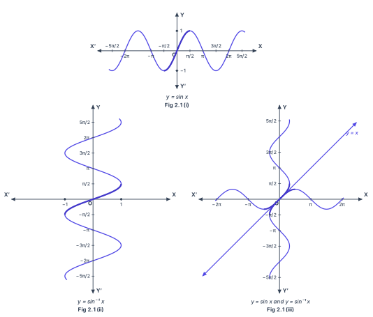
If is invertible then , so the graph of is obtained from the graph of sine by interchanging the and axes: a point on the sine graph becomes . Equivalently, it is the mirror image (reflection) of the sine graph in the line . The dark portion of the graph represents the principal value branch.
Inverse Cosine Function ()
Cosine has domain and range . Restricted to it is one-one and onto with range (and likewise on , , etc., giving branches). The principal value branch has range :
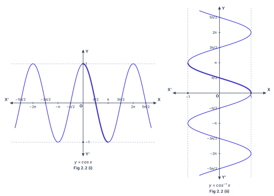
The graph of is obtained, as for , by reflecting in the line .
Inverse Cosecant Function ()
Since , cosecant has domain and range , i.e. all real values except , and is undefined at integral multiples of . Restricted to it is one-one and onto with range (other branches use , , etc.). The principal value branch gives
Inverse Secant Function ()
Since , secant has domain and range , and is undefined at odd multiples of . Restricted to it is one-one and onto with range (other branches: , , etc.). The principal value branch gives
Inverse Tangent Function ()
Tangent has domain and range , and is undefined at odd multiples of . Restricted to it is one-one and onto with range (other branches: , , etc.). The principal value branch gives
The range of is the open interval , not a closed one, because is undefined at .
Inverse Cotangent Function ()
Cotangent has domain and range , and is undefined at integral multiples of . Restricted to it is one-one and onto with range (other branches: , , etc.). The principal value branch gives
Summary Table: Principal Value Branches
| Inverse Function | Domain | Range (Principal Value Branch) |
|---|---|---|
Drawn by us to help you understand the concept clearly, and verified to make sure it's accurate. For exams, practice from your textbook's own diagram.
What Fig. 2.1 Shows
The figure is arranged as three separate coordinate panels that together tell the story of how the inverse sine function is constructed from the sine function.
Panel (i) — top centre — shows the familiar graph of . The -axis is marked at intervals of from to , and the -axis shows the range . The curve oscillates as a smooth wave between and . A thicker, darker segment of this curve is highlighted over the interval on the -axis. This dark portion is the principal-value branch of the sine function — the restricted domain on which sine becomes one-to-one.
Panel (ii) — bottom left — shows . This graph is obtained by reflecting the sine curve across the line . The domain is now on the -axis, and the -axis runs through multiples of up to . The curve rises vertically from to , then continues in repeating vertical segments. The dark portion of this curve lies between and — this is the principal value branch of .
Panel (iii) — bottom right — superimposes three graphs on the same axes: , , and the straight line (drawn with arrows at both ends). The two curves are mirror images of each other across this line. Each curve has its principal branch darkened, making the reflection relationship visually immediate.
The Core Idea
The figure teaches a fundamental principle: the graph of an inverse function is the reflection of the original function's graph across the line . This works because if lies on the graph of , then lies on the graph of . Swapping coordinates is equivalent to reflecting across .
But sine is not one-to-one on its entire domain . To define an inverse, we must restrict sine to an interval where it is one-to-one and onto . The standard choice is , shown as the dark segment in panel (i). This restricted sine is then reflected to give the principal branch of in panel (ii), with range .
The principal value branch of has domain and range . This is the only branch used unless otherwise specified.
Key Formulas Illustrated
The figure directly supports these defining relationships:
From this, two composition identities follow:
The second identity holds only when lies in the principal value range. If is outside , then gives the angle in that has the same sine as — not itself.
Do not confuse with . The notation means the inverse sine function (arcsine), while . They are completely different. …
Drawn by us to help you understand the concept clearly, and verified to make sure it's accurate. For exams, practice from your textbook's own diagram.
Understanding Fig. 2.2: The Graphs of and
The figure presents two panels side by side, showing how the cosine function and its inverse are related through reflection and domain restriction.
Panel (i):
The first panel shows the familiar cosine wave plotted on the - plane. The horizontal axis () carries -marks at intervals of , from to . Two dashed horizontal guide lines run at and , marking the maximum and minimum values of cosine. The full curve oscillates between these bounds, crossing the -axis at odd multiples of .
What makes this figure special is the darkened, thicker arc drawn over the interval . This arc runs from the point down to . This is the principal-value branch of the cosine function — the restricted portion that makes the function one-to-one. On this restricted domain , takes every value in exactly once, so it becomes invertible.
Panel (ii):
The second panel shows the inverse cosine function, obtained by reflecting the cosine curve across the line . The domain is now , indicated by dashed vertical lines at and . The -axis is marked at multiples of .
The darkened segment of this curve runs from rising to . This is the principal branch of , with range . Every point on this segment corresponds to a point on the darkened arc in panel (i), with coordinates swapped.
The principal value branch of is defined as:
This means: for any in , gives the unique angle in such that .
The Physical Idea
The figure teaches a fundamental concept about invertibility. Trigonometric functions are periodic and therefore not one-to-one over their natural domains. To define an inverse, we must restrict the domain to an interval where the function is strictly monotonic (here, decreasing from to ). The inverse function then "undoes" the original: if , then , provided lies in the principal range .
The reflection across is not just a geometric trick — it embodies the algebraic relationship between a function and its inverse. Every point on the cosine curve becomes on the inverse cosine curve.
Key Formulas Developed from This Figure
The textbook uses this graphical understanding to establish the fundamental identities:
Composition identities for cosine and its inverse
The first identity says: take any in , find its angle in , then take the cosine of that angle — you get back . The second says: take any angle in , compute , then find the inverse cosine of that value — you get back .
The second identity fails if is outside . For example, , not , because is the unique angle in whose cosine equals . Always check that the angle lies in the principal range before applying this identity.
How This Connects to Other Inverse Trigonometric Functions …
Drawn by us to help you understand the concept clearly, and verified to make sure it's accurate. For exams, practice from your textbook's own diagram.
Understanding Fig. 2.3: The Cosecant and Its Inverse
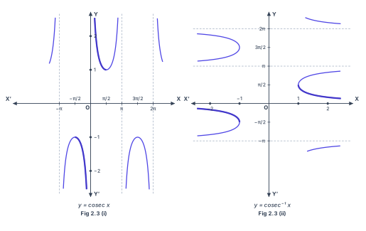
The figure presents two carefully aligned panels that show the relationship between and its inverse . The left panel displays the cosecant function itself, while the right panel shows its inverse obtained by reflecting across the line . This visual pairing is the standard method for understanding any inverse function: if lies on the graph of , then lies on the graph of .
The Left Panel:
The cosecant function is defined as , so it inherits the vertical asymptotes of the reciprocal wherever . These occur at for any integer , and the figure shows dashed vertical lines at to mark these forbidden values. Between each pair of asymptotes, the graph forms a U-shaped branch that opens upward or downward. The branches touch the lines and at their minima and maxima respectively — these are the points where , so .
The axes are labelled with key points: the -axis shows , and the -axis shows . The principal branch — the one chosen for defining the inverse — is darkened. This branch lies over the interval with the point removed. On this branch, for in we have , and for in we have .
The Right Panel:
The inverse cosecant function is defined only for , since the range of is . The graph shows horizontal dashed asymptotes at , which are the reflections of the vertical asymptotes from the left panel. The two darkened arcs correspond to the principal value branch: one arc lies in for , and the other lies in for .
The principal value branch of has range , which is exactly the same as the restricted domain chosen for to make it one-to-one. This symmetry is the entire point of the figure.
The Key Formula
The fundamental relationship that the figure illustrates is:
This means that finding asks: "What angle in the principal range has cosecant equal to ?" The figure makes this concrete by showing how each point on the darkened branch of maps to a corresponding point on the darkened branch of through reflection across .
Why This Matters for Problem Solving
When you encounter in an exam, the figure reminds you of three critical facts:
- The domain is — never try to evaluate for values between and . …
Drawn by us to help you understand the concept clearly, and verified to make sure it's accurate. For exams, practice from your textbook's own diagram.
Understanding Fig. 2.4: The secant and inverse secant pair
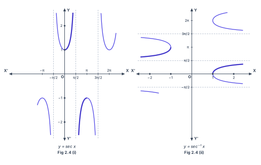
The figure presents two coordinated panels that show how the secant function and its inverse are related through reflection across the line . This visual relationship is the same geometric principle that connects any function with its inverse — a concept introduced in Chapter 1 and now applied to trigonometric functions.
Panel (i):
The secant function, defined as , has a domain that excludes all odd multiples of — these are the points where . The graph shows vertical dashed asymptotes at , , and , marking where the function blows up to .
The curve consists of repeating U-shaped branches. Each branch opens upward (touching at its minimum) or downward (touching at its maximum), depending on the interval. The -axis is marked at , , , , , and ; the -axis shows , , , and .
The principal branch — the one we restrict to make the function one-to-one — is darkened. This branch lies over the interval with the point removed. On , the curve rises from upward toward the asymptote; on , it rises from upward (becoming less negative) toward the asymptote. This restricted secant function is one-to-one and covers all values .
Panel (ii):
The inverse secant function is obtained by reflecting the principal branch of across the line . Its domain is , matching the range of the restricted secant. The range of is , which corresponds to the restricted domain of the secant.
The graph shows horizontal dashed asymptotes at , , and , which are the reflections of the vertical asymptotes from the secant graph. The principal arcs are darkened: for , the curve lies in ; for , it lies in .
The key insight is that the principal value branch of excludes from its range, just as the principal branch of excludes from its domain. This ensures the inverse function is well-defined and single-valued.
The central formula
The defining relationship between secant and its inverse is:
Here, is any real number with magnitude at least , and is the angle (in radians) whose secant equals , taken from the principal value branch. The restriction is what makes the correspondence one-to-one — without it, infinitely many angles would give the same secant value.
What the figure teaches …
Drawn by us to help you understand the concept clearly, and verified to make sure it's accurate. For exams, practice from your textbook's own diagram.
What Fig. 2.5 Shows
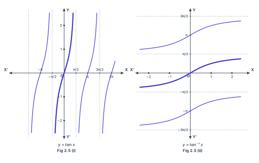
The figure is split into two panels placed side by side, showing how the tangent function and its inverse are related through reflection.
Panel (i): — the familiar repeating curve with vertical dashed asymptotes at , , , . The -axis is marked at , , , , , ; the -axis at , , , . Each branch of the curve rises steeply from to between consecutive asymptotes. The central branch over , passing through the origin, is drawn in a darker line — this is the principal branch chosen for inversion.
Panel (ii): — the reflection of the principal branch across the line . It is an increasing S-shaped curve defined for all real , with horizontal dashed asymptotes at . The curve passes through the origin, and its range is exactly . The other branches of (the lighter curves in panel i) reflect to corresponding branches of at , etc., but these are not part of the principal value.
The Core Idea
A function must be one-to-one to have an inverse. The tangent function on its full domain is not one-to-one — it repeats every and blows up at odd multiples of . By restricting to the open interval , we obtain a bijection onto . The inverse of this restricted function is , also written .
The textbook defines the principal value branch as:
This means: for any real number , is the unique angle in such that .
Key Relationships from the Figure
The reflection property gives two fundamental identities:
The second identity is the reason the principal branch is chosen: it ensures that applying after returns the original angle, but only when that angle lies in the restricted interval. If is outside , gives the angle in the principal branch that has the same tangent — not the original .
A common mistake: is not true for all . For example, , not . Always check that the angle lies in .
What the Asymptotes Tell Us …
Drawn by us to help you understand the concept clearly, and verified to make sure it's accurate. For exams, practice from your textbook's own diagram.
What Fig. 2.6 Shows
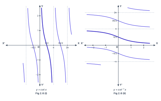
The figure has two panels, placed side by side, that together illustrate how the inverse cotangent function is constructed from the original cotangent function.
Panel (i): — the familiar cotangent curve. The horizontal axis is , the vertical axis is . The graph consists of infinitely many repeating branches, each decreasing from left to right. Vertical dashed lines (asymptotes) appear at every integer multiple of : . The curve crosses the -axis at . The axes are marked at and at . One particular branch — the one lying over the open interval — is drawn more darkly than the others. This darkened branch passes through the point and is called the principal branch of .
Panel (ii): — the inverse cotangent function. This graph is obtained by reflecting the principal branch of across the line . The axes are now swapped: the horizontal axis is , the vertical axis is . The curve is defined for all real (the entire -axis) and is strictly decreasing. Horizontal dashed lines (asymptotes) appear at . The darkened central branch — the one that corresponds to the reflection of the principal branch from panel (i) — runs between and , passing through the point . This darkened branch is the principal value branch of .
The principal value branch of is the only branch that is used as the standard inverse cotangent function. Its range is , not including the endpoints.
The Physical Idea
The figure teaches a fundamental concept about inverse functions: to define an inverse for a periodic function like , we must first restrict the original function to an interval where it is one-to-one (bijective). The cotangent function on its full domain is not one-to-one — it repeats every units. But if we restrict it to the open interval , it becomes strictly decreasing and covers every real number exactly once. This restricted function has an inverse, and that inverse is .
The reflection across is the geometric way of swapping the roles of input and output. Every point on the principal branch of becomes the point on the principal value branch of . For example, on becomes on .
Key Formulas
The textbook establishes the following central relationships from this figure:
This notation means: the inverse cotangent function takes any real number as input and returns an angle in the open interval as output. The domain is all real numbers; the range (principal value branch) is .
The defining relation is:
In words: if is the inverse cotangent of , then is the angle in whose cotangent equals .
Two important composition identities follow directly:
The first says: take any real , find its inverse cotangent (an angle in ), then take the cotangent of that angle — you get back . The second says: start with any angle in , take its cotangent, then take the inverse cotangent of that result — you get back . …
| Function | Domain | Range (principal value branch) |
|---|---|---|