Physics · Ch 2 — Motion in a Straight Line

Kinematic Equations for Uniformly Accelerated Motion

2.4

Kinematic Equations for Uniformly Accelerated Motion

Concept First: Why We Need These Equations

When acceleration is constant, the motion is simple enough that we can write exact relationships between position, velocity, acceleration, and time. These relationships are called the kinematic equations. They are not new physics — they follow directly from the definitions of velocity and acceleration, integrated under the condition that acceleration does not change.

The key insight: if acceleration is constant, then velocity changes linearly with time, and position changes quadratically with time. Every result in this section flows from those two facts.

Deriving the First Equation: $v = v_0 + at$

Start from the definition of acceleration for one-dimensional motion:

a = \frac{dv}{dt}

Since $a$ is constant, we can integrate both sides from the initial instant $t=0$ (where velocity is $v_0$ ) to any later time $t$ (where velocity is $v$ ):

\int_{v_0}^{v} dv = \int_{0}^{t} a \, dt

The left side integrates to $v - v_0$ . On the right, $a$ is constant, so it comes out of the integral:

v - v_0 = a \int_{0}^{t} dt = a t

Therefore:

v = v_0 + at

This is the first kinematic equation. It tells us that under constant acceleration, the final velocity is the initial velocity plus the accumulated change $a t$ .

Watch out

This equation gives the velocity at time $t$ , but it says nothing about where the object is. Position requires a separate equation.

Deriving the Second Equation: $x = v_0 t + \frac{1}{2} a t^2$

The textbook derives this using the area under the $v$ - $t$ graph. This geometric approach is elegant and worth understanding.

From the definition of velocity, $v = dx/dt$ , the displacement is the area under the velocity-time curve. For uniformly accelerated motion, the $v$ - $t$ graph is a straight line from $(0, v_0)$ to $(t, v)$ .

The area under this line between $t=0$ and $t=t$ is the sum of:

a rectangle of area $v_0 t$ (the area if velocity stayed at $v_0$ )
a triangle of area $\frac{1}{2}(v - v_0)t$ (the extra area due to acceleration)

So:

x = v_0 t + \frac{1}{2}(v - v_0)t

But from the first equation, $v - v_0 = a t$ . Substituting:

x = v_0 t + \frac{1}{2}(a t) t = v_0 t + \frac{1}{2} a t^2

This is the second kinematic equation.

Note

The textbook also writes this as $x = \left(\frac{v_0 + v}{2}\right) t$ , which shows that the displacement equals the average velocity multiplied by time. For constant acceleration, the average velocity is indeed the arithmetic mean of initial and final velocities: $\bar{v} = \frac{v_0 + v}{2}$ .

Deriving the Third Equation: $v^2 = v_0^2 + 2 a x$

Eliminate time between the first two equations. From $v = v_0 + at$ , we have $t = (v - v_0)/a$ . Substitute this into $x = v_0 t + \frac{1}{2} a t^2$ :

x = v_0 \left(\frac{v - v_0}{a}\right) + \frac{1}{2} a \left(\frac{v - v_0}{a}\right)^2

x = \frac{v_0(v - v_0)}{a} + \frac{1}{2} \frac{(v - v_0)^2}{a}

Multiply through by $2a$ :

2a x = 2 v_0(v - v_0) + (v - v_0)^2

2a x = 2 v_0 v - 2 v_0^2 + v^2 - 2 v_0 v + v_0^2

2a x = v^2 - v_0^2

Therefore:

v^2 = v_0^2 + 2 a x

This is the third kinematic equation. It is especially useful when time is not known or not needed.

Tip

The third equation can also be derived directly from calculus using $a = v \frac{dv}{dx}$ , which is shown in Example 2.2. This method works even for non-uniform acceleration, though the result would then be an integral rather than a simple formula.

The Complete Set of Equations

For motion starting at $x = 0$ when $t = 0$ :

v = v_0 + at

These three equations connect the five quantities $v_0$ , $v$ , $a$ , $t$ , and $x$ . Given any three, the other two can be found.

General Form with Initial Position $x_0$

If the particle starts at position $x_0$ (not necessarily zero) at $t = 0$ , then the displacement is $x - x_0$ rather than $x$ . The equations become:

v = v_0 + at

x = x_0 + v_0 t + \frac{1}{2} a t^2

v^2 = v_0^2 + 2 a (x - x_0)

The first equation is unchanged because it involves only velocity, not position.

Calculus Derivation (Example 2.2)

The textbook shows that these equations can be obtained directly from the definitions using integration. This method is more general and works even when acceleration is not constant (though the resulting integrals may not be simple).

For velocity: $a = dv/dt$ gives $dv = a\,dt$ . Integrating:

\int_{v_0}^{v} dv = \int_{0}^{t} a\,dt = a \int_{0}^{t} dt

v - v_0 = a t \quad \Rightarrow \quad v = v_0 + a t

For position: $v = dx/dt$ gives $dx = v\,dt$ . Substituting $v = v_0 + a t$ :

\int_{x_0}^{x} dx = \int_{0}^{t} (v_0 + a t)\,dt

x - x_0 = v_0 t + \frac{1}{2} a t^2

For the third equation: Use the chain rule: $a = \frac{dv}{dt} = \frac{dv}{dx} \cdot \frac{dx}{dt} = v \frac{dv}{dx}$ . Then $v\,dv = a\,dx$ . Integrating:

\int_{v_0}^{v} v\,dv = \int_{x_0}^{x} a\,dx

\frac{v^2}{2} - \frac{v_0^2}{2} = a(x - x_0)

v^2 = v_0^2 + 2a(x - x_0)

Important

The calculus method is more powerful because it can handle non-uniform acceleration. If $a$ is a function of time, the integral $\int a\,dt$ must be evaluated explicitly rather than simply becoming $a t$ .

Free Fall: A Special Case of Uniform Acceleration

An object in free fall (neglecting air resistance) experiences constant acceleration $g = 9.8 \text{ m/s}^2$ downward. If we choose the upward direction as positive, then $a = -g$ .

For an object released from rest ( $v_0 = 0$ ) at $y = 0$ :

v = -g t = -9.8 t \text{ m/s}

y = -\frac{1}{2} g t^2 = -4.9 t^2 \text{ m}

v^2 = -2 g y = -19.6 y \text{ m}^2/\text{s}^2

The negative signs indicate downward motion. The magnitude of velocity increases with time, even though the acceleration is negative — this is because the velocity and acceleration are in the same direction (both downward).

Watch out

A common mistake is to think that negative acceleration always means slowing down. It does not. Negative acceleration means acceleration in the negative direction. If velocity is also negative, the object speeds up.

Galileo's Law of Odd Numbers (Example 2.5)

For a body falling from rest, the distances travelled in successive equal time intervals are in the ratio $1 : 3 : 5 : 7 : \ldots$ .

Proof: For free fall from rest, $y = \frac{1}{2} g t^2$ (taking downward as positive for simplicity). Divide time into intervals of length $\tau$ . The positions at times $0, \tau, 2\tau, 3\tau, \ldots$ are:

Time	Position $y$	In units of $y_0 = \frac{1}{2}g\tau^2$	Distance in that interval
$0$	$0$	$0$	—
$\tau$	$\frac{1}{2}g\tau^2$	$1$	$1$
$2\tau$	$\frac{1}{2}g(2\tau)^2 = 4 \cdot \frac{1}{2}g\tau^2$	$4$	$3$
$3\tau$	$\frac{1}{2}g(3\tau)^2 = 9 \cdot \frac{1}{2}g\tau^2$	$9$	$5$
$4\tau$	$\frac{1}{2}g(4\tau)^2 = 16 \cdot \frac{1}{2}g\tau^2$	$16$	$7$

Figure 2.5Area under v-t curve for an object with uniform acceleration.

Fig. 2.5 — Area under v-t curve for an object with uniform acceleration.

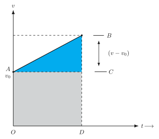
Drawn by us to help you understand the concept clearly, and verified to make sure it's accurate. For exams, practice from your NCERT textbook's own diagram.

The figure is a velocity–time graph for an object moving with uniform acceleration. The vertical axis is velocity $v$ , the horizontal axis is time $t$ . The graph is a straight line sloping upward from point A on the velocity axis to point B. Point A lies at $v = v_0$ (the initial velocity) on the $v$ -axis, and point B is somewhere higher up the line, corresponding to a later time $t$ . The line’s constant slope tells you the acceleration $a$ is constant.

The area under the entire line from $t = 0$ to $t = t$ is divided into two parts. A rectangle OACD sits below the horizontal line through A — its height is $v_0$ and its width is $t$ , so its area is $v_0 t$ . Above that rectangle, a triangle ABC sits between the line and the $v_0$ level. The triangle’s base is $t$ and its vertical height is the difference $v - v_0$ marked on the right edge. Its area is $\frac{1}{2} t (v - v_0)$ .

The physical idea is that the area under a velocity–time graph gives the displacement of the object. For uniform acceleration, the total displacement $s$ is the sum of these two areas:

s = v_0 t + \frac{1}{2} t (v - v_0)

But since acceleration $a = \frac{v - v_0}{t}$ , we have $v - v_0 = a t$ . Substituting that into the triangle’s area gives the familiar kinematic equation:

s = v_0 t + \frac{1}{2} a t^2

Here $s$ is the displacement, $v_0$ the initial velocity, $a$ the constant acceleration, and $t$ the time elapsed. The rectangle accounts for the distance the object would have covered if it kept moving at its initial speed; the triangle accounts for the extra distance gained because it is speeding up.

Important

This figure is the geometric foundation for the second equation of motion. The same graph also yields the first equation $v = v_0 + a t$ directly from the slope, and the third equation $v^2 = v_0^2 + 2 a s$ by eliminating $t$ between the area and slope relations. …

Start your 14-day free trial to unlock the full solution →

← Previous · 2.3Acceleration Next · 2.4 →Example 2.2 — Obtain equations of motion for constant acceleration using method of c…

Kinematic Equations for Uniformly Accelerated Motion