Q.Solve the following Linear Programming Problem Graphically. Maximize Subject to , and
Plot the feasible region defined by the constraints, identify the corner points, evaluate the objective function at each vertex, and select the maximum. The optimal solution is with maximum value .
Why the graphical method works
Linear programming finds the best outcome (maximum or minimum) of a linear objective function subject to linear constraints. The fundamental theorem tells us that if an optimal solution exists, it must occur at a corner point (vertex) of the feasible region. This is because the objective function is a plane, and as we slide it across the feasible region, the last point of contact before leaving the region is always a vertex.
For two-variable problems, we can visualize this geometrically: plot each constraint as a boundary line, shade the feasible side, find where they all overlap, then test the corners.
Step-by-step solution
1. Convert inequalities to boundary equations
Each constraint inequality becomes an equation for its boundary line:
- (simplifies to )
- (vertical line at )
- (horizontal line at )
- (the -axis)
- (the -axis)
2. Find intercepts for each boundary
For :
- When : , giving point
- When : , giving point
For : vertical line through and for all
For : horizontal line through and for all
3. Determine the feasible region
Test a point (say the origin) in each inequality to find which side is feasible:
- ✓ (origin side is feasible)
- ✓ (left of the line)
- ✓ (below the line)
- , (first quadrant)
The feasible region is the intersection of all these half-planes in the first quadrant.
4. Identify corner points
The vertices of the feasible region occur where boundary lines intersect:
| Intersection of | Coordinates | Check feasibility |
|---|---|---|
| , | All constraints satisfied ✓ | |
| , | Check: ✓ | |
| , | Check: ✗ | |
| , | All constraints satisfied ✓ | |
| , | Check: ✗ | |
| , | ✓; ✓ | |
| , | ✓; ✓ | |
| , | Check: ✗ |
Not every intersection of two boundary lines is a corner of the feasible region. Always verify that the point satisfies all constraints before including it.
The valid corner points are: , , , , and .
5. Evaluate the objective function at each corner
| Corner point | |
|---|---|
6. Select the maximum
The maximum value of is , occurring at the point .
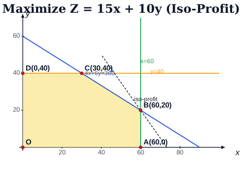
Sliding the iso-profit line up-right across the bounded pentagon, the maximum Z = 1100 is reached at B(60, 20).
In graphical LP, once you've plotted the feasible region, you can also visualize the objective function as a family of parallel lines for different values of . Slide this line outward (for maximization) until it just touches the last corner of the feasible region.
The maximum value is at .
Unlock everything free for 14 days
- Full step-by-step solutions
- Concept-first explanations
- Methods, shortcuts & mistakes
- PYQ mapping + timed mock tests
Full access for 14 days. No credit card required.