Physics · Ch 2 — Electrostatic Potential and Capacitance

Potential Due to a Point Charge

2.3

Potential Due to a Point Charge

Concept First

The electric potential at a point due to a point charge is the work done per unit positive test charge in bringing it from infinity to that point, against the electrostatic force. This is a scalar quantity that depends only on the distance from the charge, not on the path taken.

Derivation of Potential Due to a Point Charge

Consider a point charge $Q$ placed at the origin. For definiteness, take $Q > 0$ . We want the potential at a point $P$ at distance $r$ from the origin.

Path Choice: Since work done is independent of path, we choose the simplest path — a straight radial line from infinity to $P$ .
Force at an Intermediate Point: At an intermediate point $P'$ at distance $r'$ from the origin, the electrostatic force on a unit positive test charge ( $q = +1 \, \text{C}$ ) is repulsive (since $Q > 0$ ). Its magnitude is given by Coulomb's law:

F = \frac{1}{4\pi\varepsilon_0} \frac{Q}{r'^2}

The force is directed radially outward along the unit vector $\hat{r}'$.

3. Work Done Against the Force: To move the test charge inward by a small displacement $\Delta r'$ (which is negative, since $r'$ decreases), the external agent must apply a force equal and opposite to the electrostatic force. The small work done by the external force is:

\Delta W = -F \, \Delta r' = -\frac{1}{4\pi\varepsilon_0} \frac{Q}{r'^2} \Delta r'

The negative sign ensures that when $\Delta r' < 0$ (moving inward), $\Delta W$ is positive (work is done *against* the field).

4. Total Work (Integration): The total work $W$ done by the external force in bringing the test charge from infinity ( $r' = \infty$ ) to the point $P$ ( $r' = r$ ) is obtained by integrating:

W = \int_{\infty}^{r} -\frac{1}{4\pi\varepsilon_0} \frac{Q}{r'^2} \, dr'

Evaluating the integral:

W = -\frac{Q}{4\pi\varepsilon_0} \int_{\infty}^{r} \frac{dr'}{r'^2} = -\frac{Q}{4\pi\varepsilon_0} \left[ -\frac{1}{r'} \right]_{\infty}^{r} = \frac{Q}{4\pi\varepsilon_0} \left( \frac{1}{r} - \frac{1}{\infty} \right)

W = \frac{1}{4\pi\varepsilon_0} \frac{Q}{r}

Definition of Potential: By definition, the electric potential $V(r)$ at point $P$ is this work done per unit positive test charge. Therefore:

V(r) = \frac{1}{4\pi\varepsilon_0} \frac{Q}{r}

Key Points About the Formula

Sign of $Q$ : The formula $V(r) = \frac{1}{4\pi\varepsilon_0} \frac{Q}{r}$ $V (r) = \frac{1}{4 π ε _{0}} \frac{Q}{r}$ holds for any sign of $Q$ $Q$ .
- If $Q > 0$ , then $V(r) > 0$ . Work is done against the repulsive force.
- If $Q < 0$ , then $V(r) < 0$ . The work done by the external force is negative, meaning the electrostatic force itself does positive work (attraction) in bringing the test charge from infinity.
Zero at Infinity: The formula is consistent with the convention that potential at infinity is zero ( $V(\infty) = 0$ ).
Nature of Potential: Potential is a scalar quantity. It varies as $1/r$ , while the electric field $E$ varies as $1/r^2$ .

Example: Calculating Potential and Work …

Figure 2.3Work done in bringing a unit positive test charge from infinity to the point P, against the repulsive force of charge Q (Q > 0), is the potential at P due to the charge Q.

Fig. 2.3 — Work done in bringing a unit positive test charge from infinity to the point P, against the repulsive force of charge Q (Q > 0), is the potential at P due to the charge Q.

Drawn by us to help you understand the concept clearly, and verified to make sure it's accurate. For exams, practice from your NCERT textbook's own diagram.

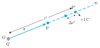
The figure illustrates the calculation of electrostatic potential due to a point charge $Q > 0$ placed at the origin O. The central idea is to find the work done by an external agent in bringing a unit positive test charge ( $+1 \, \text{C}$ ) from infinity to a point P, against the repulsive Coulomb force.

What the diagram shows

Origin O is at the lower-left, with the charge $Q$ (positive) marked below the label O.
A straight radial ray extends from O to the upper-right, representing the path along which the test charge is moved.
On this ray, two points are marked: P (closer to O) and P′ (farther from O, between P and infinity). The vector from O to P is labelled $\mathbf{r}$ , and from O to P′ is labelled $\mathbf{r}'$ .
A small segment between P and P′ is highlighted with a dashed double-arrow and labelled $\Delta r'$ — this represents an infinitesimal displacement along the radial direction.
At the far end of the ray, beyond P′, the line is dashed and labelled ∞, with a +1 C symbol indicating the unit positive test charge initially at infinity.

Physical idea taught

The figure visualizes the path-independent nature of work done by an external force. Since the electrostatic force is conservative, we choose the simplest path: straight along the radial direction. The test charge is brought from infinity (where potential is zero by convention) to point P. At each intermediate point P′, the repulsive force on the test charge is given by Coulomb's law. The external agent must apply an equal and opposite force to move the charge slowly (without acceleration). The work done in moving the test charge through a small radial displacement $\Delta r'$ (from P′ toward O) is positive because the displacement is opposite to the repulsive force.

Key formula derived

The work done by the external force in moving the unit positive test charge from infinity to P is obtained by integrating the infinitesimal work contributions:

W = \int_{\infty}^{r} \frac{Q}{4\pi\varepsilon_0 r'^2} \, (-dr') = \frac{Q}{4\pi\varepsilon_0 r}

Here:

$Q$ = source charge at the origin (positive in this case)
$\varepsilon_0$ = permittivity of free space
$r'$ = distance from origin to the intermediate point P′
$r$ = distance from origin to the final point P …

Figure 2.4Variation of potential V with r and field E with r for a point charge Q.

Fig. 2.4 — Variation of potential V with r and field E with r for a point charge Q.

Drawn by us to help you understand the concept clearly, and verified to make sure it's accurate. For exams, practice from your NCERT textbook's own diagram.

What the Graph Shows

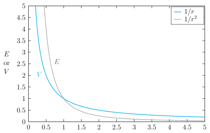
The figure is a single 2‑D line graph that plots two physical quantities — electric field $E$ and electrostatic potential $V$ — against the radial distance $r$ from a point charge $Q$ (taken positive).

Horizontal axis ( $r$ ): Distance from the charge, scaled from 0 to 5 (arbitrary units).
Vertical axis (“ $E$ or $V$ ”): Both $E$ and $V$ are plotted on the same scale, with ticks from 0 to 5 in steps of 0.5.

Two curves fall steeply from the upper‑left corner and flatten as they approach the horizontal axis:

Black curve (steeper): Represents the electric field $E \propto 1/r^2$ .
Blue curve (less steep): Represents the potential $V \propto 1/r$ .

A small legend box identifies the curves with “— $1/r$ ” (for $V$ ) and “— $1/r^2$ ” (for $E$ ).

Key Physical Idea

The graph visually compares how fast $E$ and $V$ decrease as you move away from the charge.

Near the origin (small $r$ ): The $1/r^2$ curve (field) lies above the $1/r$ curve (potential) — the field falls off more rapidly.
At large $r$ : The $1/r$ curve (potential) lies above the $1/r^2$ curve — the potential decays more slowly than the field.

This difference in decay rates is why, for example, the potential at a point is easier to measure than the field at large distances: $V$ remains appreciable even where $E$ has become very small.

The Formula Behind the Graph

From the textbook derivation, the potential at a distance $r$ from a point charge $Q$ is

V(r) = \frac{1}{4\pi\varepsilon_0} \frac{Q}{r}

where:

$Q$ = magnitude of the point charge (positive in the figure),
$r$ = distance from the charge,
$\varepsilon_0$ = permittivity of free space,
$\frac{1}{4\pi\varepsilon_0} \approx 9 \times 10^9\ \text{N m}^2/\text{C}^2$ .

The corresponding electric field is

E(r) = \frac{1}{4\pi\varepsilon_0} \frac{Q}{r^2}

The graph shows the functional forms $V \propto 1/r$ and $E \propto 1/r^2$ — the constants $\frac{Q}{4\pi\varepsilon_0}$ simply scale the curves vertically.

What the Figure Teaches …

Start your 14-day free trial to unlock the full solution →

← Previous · 2.2Electrostatic Potential Next · 2.3 →Example 2.1 — (a) Calculate the potential at a point P due to a charge of 4 × 10⁻⁷C …