Normal Distribution: Shape and Properties

The binomial and Poisson distributions both describe a random variable that can only take whole-number values — a batch can have 2 defectives or 3, never 2.4. Many business and natural variables, however, are continuous — they can, at least in principle, take any value on a scale: the exact daily sales figure of a shop, the height or weight of individuals, the marks scored by a large batch of students, or the error in a precise measurement. The theoretical distribution most commonly used to model such variables is the normal distribution, sometimes called the Gaussian distribution.

The normal distribution's probability density function (p.d.f.) is:

where $\mu$ is the mean and $\sigma$ is the standard deviation of the distribution. This formula does not need to be derived for this syllabus — what matters is its shape and the properties that follow from it:

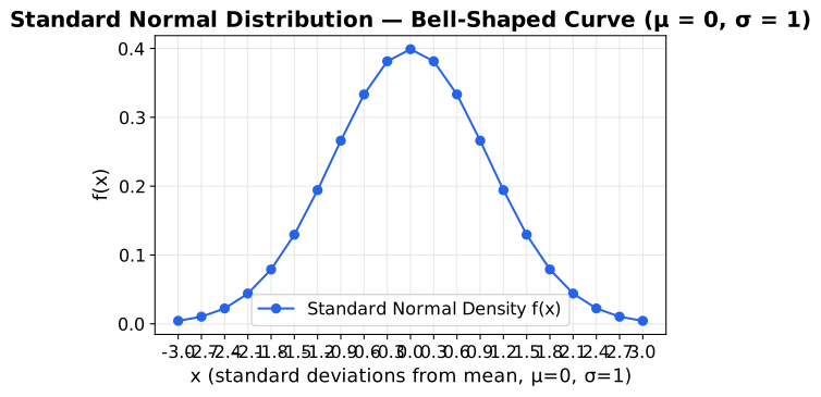
• The curve is bell-shaped and perfectly symmetric about the mean $\mu$.
• Mean = Median = Mode, all located at the centre of the curve.
• The total area under the curve equals $1$, since it represents the total probability.
• The curve is asymptotic to the x-axis — its tails extend indefinitely in both directions and never actually touch zero.
• The overall shape is controlled entirely by $\sigma$: a small $\sigma$ gives a tall, narrow curve (values cluster close to the mean); a large $\sigma$ gives a short, wide curve (values are more spread out).

…