Physics · Ch 13 — Kinetic Theory

Behaviour of Gases

13.3

Behaviour of Gases

12.3 Behaviour of Gases

Section 12.2 introduced the ideal gas law, $PV = \mu RT$ , as a macroscopic fact about gases — a relation between pressure, volume, temperature and the amount of substance that every real gas obeys, to a very good approximation, at ordinarily low densities. This section looks more closely at where that law comes from experimentally, how it leads to a new fundamental constant of nature — the Boltzmann constant — and how the two classical gas laws, Boyle's law and Charles' law, are simply special cases of it.

The Empirical Law PV = KT

Careful experiments on a fixed quantity of gas — the same sample, the same number of molecules, throughout — show that the product of its pressure and volume is directly proportional to its absolute temperature:

PV = KT \qquad \text{...(12.1)}

Here $K$ is a constant for that particular sample of gas. It is not a universal constant — its value depends on how much gas is present: twice as many molecules of the same gas, held at the same pressure and temperature, occupy twice the volume, so $K$ doubles.

Note

Equation (12.1) is a purely empirical summary of what Boyle and Charles found by experiment in the seventeenth and eighteenth centuries, long before anyone knew gases were made of molecules. Kinetic theory (Section 12.4) later derives this same law from the mechanics of colliding molecules — but historically, the experimental law came first, and the molecular explanation came almost two centuries later.

The Boltzmann Constant

What exactly does $K$ depend on? Take two different samples of gas — they can even be two chemically different gases — in states $(P_1, V_1, T_1)$ and $(P_2, V_2, T_2)$ , containing $N_1$ and $N_2$ molecules respectively. Experiment shows that:

\frac{P_1 V_1}{N_1 T_1} = \frac{P_2 V_2}{N_2 T_2} = \text{constant} \qquad \text{...(12.2)}

In other words, $K$ is simply proportional to the number of molecules present, $K = N k_B$ , where $k_B$ is a single constant — the same for every gas, regardless of its chemical identity. This universal constant is called Boltzmann's constant:

k_B = 1.38 \times 10^{-23} \ \text{J K}^{-1}

With this, Equation (12.1) can be written in its molecular form, $PV = N k_B T$ — the exact relation used in Section 12.4 to connect pressure to the mean square speed of gas molecules. That $k_B$ does not depend on whether the gas is helium, oxygen, or carbon dioxide is itself an important clue: it tells us pressure and temperature are governed only by how many molecules are present and how energetically they move, never by what those molecules are chemically.

The Ideal (or Perfect) Gas

A real gas obeys $PV = KT$ only approximately, and the approximation improves as the gas is made more dilute. This motivates a precise, idealised definition:

Important

An ideal gas (or perfect gas) is one that satisfies

$PV = \mu RT$

exactly, at every pressure and temperature. Here $\mu$ is the number of moles of gas present, and $R$ is the universal gas constant, $R = 8.31\ \text{J mol}^{-1}\text{K}^{-1}$ — the same value for every gas.

No real gas is perfectly ideal, but at low pressures and high temperatures, real gases approach ideal behaviour very closely, because the molecules are then far enough apart that intermolecular forces and the molecules' own finite volume both become negligible.

Boyle's Law

At constant temperature, the ideal gas equation reduces to the relation Robert Boyle discovered experimentally in 1662:

PV = \text{constant}

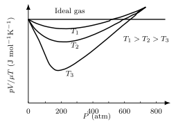
The accompanying figure (Figure 12.1) tests this directly against real gas data: it plots the quantity $pV/\mu T$ — which equals $R$ exactly for an ideal gas, at every pressure — against pressure $p$ , for three fixed temperatures $T_1 > T_2 > T_3$ . If gases were perfectly ideal, all three curves would lie exactly on the horizontal dashed line at $R = 8.314\ \text{J mol}^{-1}\text{K}^{-1}$ . Instead, each curve dips below that line at moderate pressure — attractive forces between molecules pull the measured pressure below the ideal prediction — and rises above it at high pressure, where the molecules' own finite size becomes significant. Every curve does, however, converge onto the ideal-gas line as $p \to 0$ : this is exactly the sense in which the ideal gas law is a limiting law, exact only as pressure approaches zero.

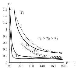
Figure 12.2 illustrates the same idea a different way, plotting $P$ directly against $V$ for steam at three temperatures. The solid curves are the real, measured isotherms; the dotted curves are what Boyle's law predicts ( $P \propto 1/V$ ) at the same temperatures. At the two higher temperatures, the solid and dotted curves lie close together — steam behaves nearly ideally there. At the lowest temperature, the solid curve visibly departs from the dotted hyperbola and flattens out at small volume, a sign that the gas is beginning to condense into a liquid rather than continuing to obey Boyle's law.

Note

Boyle's law, like Charles' law below, is not an independent postulate — it is simply the ideal gas equation $PV = \mu RT$ with $T$ (and $\mu$ ) held fixed.

Charles' Law

At constant pressure, the same ideal gas equation instead gives the relation Jacques Charles established experimentally around 1787:

V \propto T

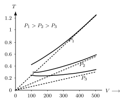
Figure 12.3 tests this for carbon dioxide. The graph plots temperature $T$ on the vertical axis (in units of 300 K) against volume $V$ on the horizontal axis (in units of 0.13 litres), for three fixed pressures $P_1 > P_2 > P_3$ . For each pressure, a dotted straight line through the origin shows what Charles' law predicts — since $V \propto T$ at fixed $P$ is a straight line through the point $V = 0,\ T = 0$ — while the solid curve alongside it shows how CO₂ actually behaves. At high temperature the real gas tracks its straight line closely; as temperature falls, the solid curve bends away from the dotted line, and the deviation is largest for the highest pressure, $P_1$ .

Important

The dotted lines all pass through the origin because Charles' law predicts $V \to 0$ as $T \to 0$ . Real gases never actually get there — they liquefy at some positive temperature well before absolute zero — which is exactly why the solid curves peel away from the straight dotted lines at low temperature. This is one of the classic experimental hints that absolute zero, though a perfectly well-defined limit, can never actually be reached by cooling a real gas.

Mixture of Non-Reactive Ideal Gases — Dalton's Law

Ideal gas behaviour extends naturally to mixtures of gases that do not chemically react with one another — ordinary air, for instance, is mostly a mixture of nitrogen and oxygen, and still obeys the ideal gas law as a whole. If $\mu_1$ moles of one gas are mixed with $\mu_2$ moles of a second, non-reacting gas, and so on, all sharing the same container of volume $V$ at the same temperature $T$ , the mixture obeys:

PV = (\mu_1 + \mu_2 + \cdots)\, RT

Equivalently, because each gas behaves exactly as it would if it alone occupied the container, the total pressure is simply the sum of the pressures each gas would exert on its own:

P = P_1 + P_2 + \cdots

Figure 12.1Real gases approach ideal gas behaviour at low pressures and high temperatures.

Fig. 12.1 — Real gases approach ideal gas behaviour at low pressures and high temperatures.

Drawn by us to help you understand the concept clearly, and verified to make sure it's accurate. For exams, practice from your textbook's own diagram.

The figure plots the quantity $\frac{pV}{\mu T}$ on the vertical axis against pressure $p$ on the horizontal axis. The vertical axis has units of J mol⁻¹ K⁻¹ — it is essentially the gas constant per mole, $R$ , for the gas being studied. The horizontal axis runs from 0 to about 800 atm. A horizontal dashed line is drawn across the graph at the value $R = 8.314$ J mol⁻¹ K⁻¹, labelled "Ideal gas". This is the reference: for an ideal gas, $\frac{pV}{\mu T} = R$ at every pressure.

Three curved lines, labelled $T_1$ , $T_2$ , and $T_3$ , are superimposed on the same axes. These are isotherms — each one shows how $\frac{pV}{\mu T}$ changes with pressure for a real gas at a fixed temperature. The temperatures satisfy $T_1 > T_2 > T_3$ . At very low pressures (near $p = 0$ ), all three curves converge to the ideal-gas line. As pressure increases, each curve dips below the ideal line, reaches a minimum, and then rises again, crossing the ideal line from below at some higher pressure. The deepest dip belongs to the lowest temperature, $T_3$ ; the shallowest dip belongs to the highest temperature, $T_1$ .

Note

The quantity $\frac{pV}{\mu T}$ is the molar gas constant only for an ideal gas. For a real gas, it deviates from $R$ because intermolecular forces and finite molecular size become important at higher pressures.

The physical idea is straightforward. At very low pressures, gas molecules are so far apart that intermolecular attractions are negligible and the volume occupied by the molecules themselves is a tiny fraction of the container volume — the gas behaves ideally. As pressure rises, molecules are pushed closer together. Attractive forces between molecules reduce the pressure exerted on the walls (compared to an ideal gas), so $pV$ is smaller than $RT$ for a given amount — hence the dip below the ideal line. At still higher pressures, the finite size of molecules becomes dominant: the molecules themselves occupy a significant fraction of the total volume, so the available free volume is less than $V$ , and $pV$ becomes larger than $RT$ — hence the rise above the ideal line.

The depth of the dip depends on temperature. At higher temperatures, molecules move faster and spend less time near each other, so the effect of attractive forces is weaker — the dip is shallower. At lower temperatures, attractions are more effective, so the dip is deeper. This is why $T_3$ (the coldest isotherm) dips the most.

The textbook uses this figure to motivate the van der Waals equation, which corrects the ideal gas law for these two effects:

\left( p + \frac{a\mu^2}{V^2} \right) \left( V - \mu b \right) = \mu RT

Here, $p$ is the pressure, $V$ the volume, $\mu$ the number of moles, $T$ the absolute temperature, and $R$ the universal gas constant. The term $\frac{a\mu^2}{V^2}$ is a correction for intermolecular attraction: it adds to the measured pressure because attractions reduce the wall-collision frequency. The term $\mu b$ is a correction for the finite volume of the molecules themselves: $b$ is the excluded volume per mole, so the available free volume is $V - \mu b$ . The constants $a$ and $b$ are different for each gas and are determined experimentally. …

Figure 12.2Experimental P-V curves (solid lines) for steam at three temperatures compared with Boyle's law (dotted lines). P is in units of 22 atm and V in units of 0.09 litres.

Fig. 12.2 — Experimental P-V curves (solid lines) for steam at three temperatures compared with Boyle's law (dotted lines). P is in units of 22 atm and V in units of 0.09 litres.

Drawn by us to help you understand the concept clearly, and verified to make sure it's accurate. For exams, practice from your textbook's own diagram.

The figure plots pressure $P$ on the vertical axis against volume $V$ on the horizontal axis. The pressure axis runs from 0 to about 1.6, in units where 1 corresponds to 22 atm. The volume axis runs from about 20 to 220, in units where 1 corresponds to 0.09 litres. Three pairs of curves appear, one above the other, each pair consisting of a solid experimental curve and a dotted theoretical curve. The three pairs correspond to three different temperatures, labelled $T_1$ , $T_2$ , and $T_3$ , with $T_1 > T_2 > T_3$ . The top pair belongs to $T_1$ , the middle pair to $T_2$ , and the bottom pair to $T_3$ .

Each solid curve shows the actual $P$ – $V$ behaviour of steam at that fixed temperature. Each dotted curve shows the prediction of Boyle's law — that is, $P \propto 1/V$ — for the same temperature. For $T_1$ and $T_2$ , the solid and dotted curves lie close together: the experimental data follow Boyle's law reasonably well. For $T_3$ , the lowest temperature, the solid curve first dips below the dotted curve and then flattens out at low volume, deviating strongly from the Boyle's law prediction.

Important

The key physical idea is that real gases obey Boyle's law only at sufficiently high temperatures. As temperature decreases, deviations become significant, especially at high pressures (low volumes). At the lowest temperature shown, the gas even begins to approach liquefaction — the flattening of the curve signals that further compression no longer raises the pressure much, because the substance is condensing into a liquid.

The textbook uses this figure to motivate the need for a more accurate equation of state. The ideal gas law,

PV = nRT,

fails to describe the behaviour of real gases under all conditions. Here $P$ is pressure, $V$ is volume, $n$ is the number of moles, $R$ is the universal gas constant, and $T$ is the absolute temperature. The figure shows that while the ideal gas law works well at high $T$ (the $T_1$ and $T_2$ curves), it breaks down at low $T$ (the $T_3$ curve). This leads directly to the van der Waals equation, which corrects for intermolecular attractions and finite molecular volume:

$\left(P + \frac{a n^2}{V^2}\right)(V - n b) = n R T,$ …

Figure 12.3Experimental T-V curves (solid lines) for CO2 at three pressures compared with Charles' law (dotted lines). T is in units of 300 K and V in units of 0.13 litres.

Fig. 12.3 — Experimental T-V curves (solid lines) for CO2 at three pressures compared with Charles' law (dotted lines). T is in units of 300 K and V in units of 0.13 litres.

Drawn by us to help you understand the concept clearly, and verified to make sure it's accurate. For exams, practice from your textbook's own diagram.

The figure plots volume (V) on the horizontal axis and temperature (T) on the vertical axis. The vertical (temperature) scale runs from 0 to 1.2, but these are not ordinary kelvin — each unit equals 300 K. So a reading of 1.0 on the axis means 300 K, 0.5 means 150 K, and so on. The horizontal (volume) scale runs from 0 to 500, where each unit is 0.13 litres. A volume of 500 on the axis therefore corresponds to $500 \times 0.13 = 65$ litres.

Three pairs of lines appear, one pair for each of three different pressures: $P_1$ , $P_2$ , and $P_3$ , with $P_1 > P_2 > P_3$ . In each pair, the solid curve is the experimental data for carbon dioxide (CO₂) at that fixed pressure, and the dotted straight line is the prediction of Charles' law for the same pressure. The dotted lines all pass through the origin, because Charles' law says volume is directly proportional to absolute temperature at constant pressure: $V \propto T$ . The solid experimental curves, however, do not pass through the origin — they show a clear deviation from the straight line, especially at lower temperatures.

The physical idea is straightforward. Charles' law is an idealisation: it assumes the gas molecules occupy no volume and exert no forces on each other. Real gases like CO₂ deviate from this behaviour, and the figure shows exactly where and how. At high temperature (upper part of the graph), the solid curve and the dotted line nearly coincide — the gas behaves almost ideally. As temperature drops, the solid curve bends away from the straight line, indicating that the real gas occupies a smaller volume than Charles' law predicts for the same temperature and pressure. The deviation is more pronounced at higher pressures: the $P_1$ curve (steepest) separates from its dotted line earliest and most dramatically.

Watch out

Do not confuse the axes: the vertical axis is temperature, not pressure, and the horizontal axis is volume. The three curves are for three different constant pressures, but pressure is not plotted on either axis — it is a parameter that labels each curve.

The key formula the textbook develops from this figure is the ideal gas equation, which combines Charles' law, Boyle's law, and Avogadro's law into a single relation:

PV = nRT

Here $P$ is the pressure of the gas, $V$ is its volume, $n$ is the number of moles, $R$ is the universal gas constant ( $8.314\ \text{J mol}^{-1}\text{K}^{-1}$ ), and $T$ is the absolute temperature in kelvin. The dotted straight lines in the figure are graphical representations of Charles' law, which is a special case of this equation when $P$ and $n$ are held constant: $V = (nR/P)\,T$ , so $V$ is a linear function of $T$ with slope $nR/P$ . …

Start your 14-day free trial to unlock the full solution →

← Previous · 13.2Molecular Nature of Matter Next · 13.3 →Example 12.1 — The density of water is 1000kg m⁻³. The density of water vapour at 100…