Mathematics · Ch 14 — Probability

Probability of the Event ‘A or B’

14.2.3

Probability of the Event ‘A or B’

The Probability of ‘A or B’: $P(A \cup B)$

When two events A and B are considered together, the event ‘A or B’ means that at least one of them occurs. In set notation, this is the union $A \cup B$ . The natural question is: how do we compute $P(A \cup B)$ from the individual probabilities $P(A)$ and $P(B)$ ?

Why $P(A \cup B)$ is Not Simply $P(A) + P(B)$

Consider the experiment of tossing a fair coin three times. The sample space has 8 equally likely outcomes. Define:

$A = \{HHT, HTH, THH\}$ — the event of getting exactly two heads
$B = \{HTH, THH, HHH\}$ — the event of getting at least two heads

The union is $A \cup B = \{HHT, HTH, THH, HHH\}$ .

Since all outcomes are equally likely, each has probability $\frac{1}{8}$ . Therefore:

P(A \cup B) = \frac{1}{8} + \frac{1}{8} + \frac{1}{8} + \frac{1}{8} = \frac{4}{8} = \frac{1}{2}

Now compute $P(A) + P(B)$ :

P(A) = \frac{3}{8}, \quad P(B) = \frac{3}{8}, \quad P(A) + P(B) = \frac{6}{8} = \frac{3}{4}

Clearly $P(A \cup B) \neq P(A) + P(B)$ . The sum $\frac{3}{4}$ is larger than the true probability $\frac{1}{2}$ .

Watch out

The mistake is that outcomes $HTH$ and $THH$ belong to both A and B. When we add $P(A)$ and $P(B)$ , these common outcomes get counted twice — once in each event. The sum overcounts the probability of the intersection $A \cap B$ .

The General Addition Rule

To correct the double-counting, we subtract the probability of the overlapping part. For any two events A and B:

P(A \cup B) = P(A) + P(B) - P(A \cap B)

This is the addition theorem of probability for two events. It holds for any random experiment, regardless of whether outcomes are equally likely.

Formal Derivation (Using the Definition of Probability)

Let the sample space be $S = \{\omega_1, \omega_2, \dots, \omega_n\}$ with probabilities $p_i = P(\{\omega_i\})$ . By definition:

P(A \cup B) = \sum_{\omega_i \in A \cup B} p_i

The union can be split into three disjoint parts:

A \cup B = (A - B) \cup (A \cap B) \cup (B - A)

Since these three sets are mutually exclusive (no outcome belongs to more than one), we can add their probabilities:

P(A \cup B) = \sum_{\omega_i \in A-B} p_i + \sum_{\omega_i \in A \cap B} p_i + \sum_{\omega_i \in B-A} p_i \quad \text{... (1)}

Now write $P(A) + P(B)$ :

P(A) + P(B) = \sum_{\omega_i \in A} p_i + \sum_{\omega_i \in B} p_i

Each of A and B can be split into two disjoint parts:

$A = (A - B) \cup (A \cap B)$
$B = (B - A) \cup (A \cap B)$

Therefore:

P(A) + P(B) = \left[ \sum_{\omega_i \in A-B} p_i + \sum_{\omega_i \in A \cap B} p_i \right] + \left[ \sum_{\omega_i \in B-A} p_i + \sum_{\omega_i \in A \cap B} p_i \right]

P(A) + P(B) = \sum_{\omega_i \in A-B} p_i + \sum_{\omega_i \in A \cap B} p_i + \sum_{\omega_i \in B-A} p_i + \sum_{\omega_i \in A \cap B} p_i

Notice that the first three terms are exactly $P(A \cup B)$ from equation (1). So:

P(A) + P(B) = P(A \cup B) + P(A \cap B)

Rearranging gives the addition rule:

P(A \cup B) = P(A) + P(B) - P(A \cap B)

Alternative Derivation (Using Set Decomposition and Axiom iii)

This approach uses a different decomposition that avoids splitting into three parts.

›Proof

Write $A \cup B$ as $A \cup (B - A)$ . Since A and $B - A$ are mutually exclusive, Axiom (iii) gives:

$P(A \cup B) = P(A) + P(B - A) \quad \text{... (2)}$

Now write B as $(A \cap B) \cup (B - A)$ . Again, $A \cap B$ and $B - A$ are mutually exclusive, so:

$P(B) = P(A \cap B) + P(B - A) \quad \text{... (3)}$

Subtract equation (3) from equation (2):

$P(A \cup B) - P(B) = P(A) - P(A \cap B)$

Therefore:

…

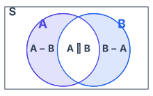
Figure 14.1Venn diagram of two events A and B showing the overlap A ∩ B

Fig. 14.1 — Venn diagram of two events A and B showing the overlap A ∩ B

Drawn by us to help you understand the concept clearly, and verified to make sure it's accurate. For exams, practice from your textbook's own diagram.

Fig. 14.1 is a Venn diagram drawn inside a rectangle labelled S, which represents the entire sample space of a random experiment. Inside the rectangle are two overlapping circles. The left circle is labelled A and is shaded indigo; the right circle is labelled B and is shaded blue. Where the two circles overlap, a central lens-shaped region is formed, and this region is labelled A ∩ B — the intersection of events A and B.

The diagram is a visual proof of the addition rule of probability. The total area of the two circles together represents $P(A) + P(B)$ . But the overlap $A \cap B$ is counted twice in that sum — once as part of A and once as part of B. To get the probability of the union $A \cup B$ (the total region covered by either circle), you must subtract the overlap once. That is the physical idea the figure teaches: the union is not simply the sum of the two events; you must correct for double-counting.

P(A \cup B) = P(A) + P(B) - P(A \cap B)

Here, $P(A \cup B)$ is the probability that event A or event B (or both) occurs. $P(A)$ and $P(B)$ are the individual probabilities of A and B. $P(A \cap B)$ is the probability that both A and B occur together — the overlap that gets subtracted.

The textbook develops this formula in two ways. First, using the coin-toss example: with three tosses, A = {HHT, HTH, THH} and B = {HTH, THH, HHH}. The outcomes HTH and THH lie in both A and B, so $P(A) + P(B) = \frac{3}{8} + \frac{3}{8} = \frac{6}{8}$ , but $P(A \cup B) = \frac{4}{8} = \frac{1}{2}$ . The difference of $\frac{2}{8}$ is exactly $P(A \cap B)$ . The Venn diagram makes this subtraction visible: the lens-shaped overlap is the region that must be removed once.

Second, the text gives a formal proof by partitioning the union into three mutually exclusive pieces: $A - B$ , $A \cap B$ , and $B - A$ . Since these three regions do not overlap, the probability of the union is the sum of their individual probabilities. Then, by writing $P(A)$ and $P(B)$ each as sums that include $P(A \cap B)$ twice, the subtraction emerges naturally. …

Start your 14-day free trial to unlock the full solution →

← Previous · 14.2.2Probabilities of Equally Likely Outcomes Next · 14.2.4 →Probability of Event ‘not A’

Probability of the Event ‘A or B’