Economics · Ch 8 — Theory of Consumer Behaviour

Elasticity and Expenditure

8.6.3

Elasticity and Expenditure

2.6.3 Elasticity and Expenditure

When a consumer buys a good, the total amount spent on it is simply the price paid multiplied by the quantity bought. This total outlay is called expenditure on the good:

E = p \times q

where $p$ is the price per unit and $q$ is the quantity demanded. A natural question arises: what happens to this expenditure when the price changes? Since price and quantity demanded move in opposite directions (the law of demand), the net effect on expenditure is not obvious. Whether total spending rises, falls, or stays the same depends entirely on how strongly quantity responds to the price change — that is, on the price elasticity of demand.

The logic in words

Consider a price increase. The higher price, by itself, pushes expenditure up. But the higher price also reduces the quantity demanded, which pulls expenditure down. Which force wins?

If the percentage drop in quantity is larger than the percentage rise in price, the quantity effect dominates and total expenditure falls.
If the percentage drop in quantity is smaller than the percentage rise in price, the price effect dominates and total expenditure rises.
If the two percentages are exactly equal, the two effects cancel out and expenditure stays unchanged.

Now consider a price decrease. A lower price, by itself, reduces expenditure. But the lower price also increases quantity demanded, which raises expenditure.

If the percentage increase in quantity is larger than the percentage fall in price, the quantity effect dominates and expenditure rises.
If the percentage increase in quantity is smaller than the percentage fall in price, the price effect dominates and expenditure falls.
If the two percentages are equal, expenditure remains unchanged.

The relationship in terms of elasticity

The price elasticity of demand, $e_D$ , is defined as:

e_D = \frac{\text{Percentage change in quantity demanded}}{\text{Percentage change in price}}

Since demand curves slope downward, $e_D$ is negative. But for the purpose of comparing magnitudes, we care about the absolute value $|e_D|$ .

Price-elastic demand ( $|e_D| > 1$ ): quantity responds more than proportionally. A price increase reduces expenditure; a price decrease raises expenditure. Expenditure moves in the opposite direction to price.
Price-inelastic demand ( $|e_D| < 1$ ): quantity responds less than proportionally. A price increase raises expenditure; a price decrease reduces expenditure. Expenditure moves in the same direction as price.
Unit-elastic demand ( $|e_D| = 1$ ): quantity responds exactly proportionally. Expenditure does not change when price changes.

Watch out

A common mistake is to think that a price increase always raises total revenue. This is only true when demand is inelastic. If demand is elastic, raising the price actually reduces total spending on the good.

A numerical illustration

The textbook presents a table with six hypothetical cases — three for a price rise and three for a price fall. Each case assumes a 10% change in price and a corresponding percentage change in quantity. The table below reproduces these cases exactly as given in the book.

Change in price ( $P$ )	% Change in price	% Change in quantity demanded ( $Q$ )	Impact on expenditure ( $P \times Q$ )	Nature of elasticity of demand
↑	+10	−8	↑	Price Inelastic
↑	+10	−12	↓	Price Elastic
↑	+10	−10	No Change	Unit Elastic
↓	−10	+15	↑	Price Elastic
↓	−10	+7	↓	Price Inelastic
↓	−10	+10	No Change	Unit Elastic

Reading the table. In row 1, price rises by 10% but quantity falls by only 8%. Since $8\% < 10\%$ , demand is inelastic and expenditure rises. In row 2, price rises by 10% but quantity falls by 12%. Since $12\% > 10\%$ , demand is elastic and expenditure falls. Row 3 shows the unit-elastic case where the two percentages are equal and expenditure is unchanged. Rows 4–6 repeat the same logic for a price fall.

The rectangular hyperbola demand curve

There is a special demand curve for which expenditure is constant at every point.

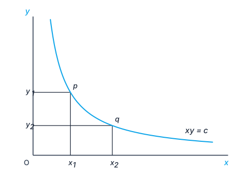
Rectangular hyperbola xy = c with two points p at (x₁, y₁) and q at (x₂, y₂), each completing a rectangle with the axes; both rectangles have the same area c.

Drawn by us to help you understand the concept clearly, and verified to make sure it's accurate. For exams, practice from your textbook's own diagram.

A rectangular hyperbola is the graph of xy = c: at every point on the curve the product of the two coordinates is the same constant c. The rectangles formed with the axes by p = (x₁, y₁) and q = (x₂, y₂) therefore have equal areas — which is why a demand curve of this shape keeps total expend …

Note

Rectangular Hyperbola

An equation of the form $xy = c$ , where $x$ and $y$ are two variables and $c$ is a constant, gives a curve called a rectangular hyperbola — a downward-sloping curve in the $x$ – $y$ plane. For any two points on the curve, the areas of the rectangles formed with the two axes are the same and equal to $c$ .

If the equation of a demand curve takes the form $p \times q = e$ , where $e$ is a constant, it is a rectangular hyperbola in which price ( $p$ ) times quantity ( $q$ ) stays constant. With such a demand curve, no matter at which point the consumer consumes, her total expenditure is always the same and equal to $e$ — which is exactly the property of unit-elastic demand.

A formal derivation of the relationship

Note

Relationship between Elasticity and Change in Expenditure on a Good

Suppose at price $p$ the demand for a good is $q$ , and at price $p + \Delta p$ the demand is $q + \Delta q$ . Expenditure changes from $pq$ to $(p + \Delta p)(q + \Delta q)$ , so the change in expenditure is

$\Delta E = (p + \Delta p)(q + \Delta q) - pq = q\Delta p + p\Delta q + \Delta p\,\Delta q$

For small values of $\Delta p$ and $\Delta q$ the product $\Delta p\,\Delta q$ is negligible, so

$\Delta E \approx q\Delta p + p\Delta q = \Delta p\left(q + p\frac{\Delta q}{\Delta p}\right)$

Since $e_D = \frac{\Delta q}{\Delta p}\cdot\frac{p}{q}$ , we have $\frac{\Delta q}{\Delta p} = e_D\cdot\frac{q}{p}$ , and therefore …

Start your 14-day free trial to unlock the full solution →

← Previous · 8.6.2Factors Determining Price Elasticity of Demand for a Good Next · key-concepts →Key Concepts