Biology · Ch 13 — Biodiversity and Conservation
Patterns of Biodiversity
Patterns of Biodiversity
The diversity of life on Earth is not spread evenly. Two major patterns help us understand where species are found and why: the latitudinal gradient in diversity and the species-area relationship.
Latitudinal Gradients
For most groups of plants and animals, species diversity decreases steadily as you move from the equator toward the poles. This is one of the best-known patterns in biogeography.
Tropical regions — the band between 23.5° N and 23.5° S latitude — contain far more species than temperate or polar areas. The numbers are striking. Colombia, which lies near the equator, has nearly 1,400 species of birds. New York, at 41° N, has only 105 species. Greenland, at 71° N, has just 56. India, with most of its land area in tropical latitudes, has more than 1,200 bird species. A tropical forest in Ecuador can have up to ten times as many species of vascular plants as a forest of equal area in the temperate Midwest of the USA.
The Amazonian rain forest in South America — largely tropical — holds the greatest biodiversity on Earth. It is home to more than 40,000 plant species, 3,000 species of fishes, 1,300 birds, 427 mammals, 427 amphibians, 378 reptiles, and over 1,25,000 invertebrates. Scientists estimate that at least two million insect species may still be waiting to be discovered and named in these forests.
Why are tropics so rich? Ecologists and evolutionary biologists have proposed three main hypotheses:
- Evolutionary time: Speciation takes time. Tropical latitudes have remained relatively undisturbed for millions of years, unlike temperate regions that experienced frequent glaciations in the past. This long, stable period has given tropical species more time to diversify.
- Constant environments: Tropical environments are less seasonal, more constant, and more predictable than temperate ones. Such stability promotes niche specialisation — species can adapt to very specific roles — which leads to greater diversity.
- Greater solar energy: The tropics receive more solar energy, which drives higher productivity. Higher productivity may indirectly support a greater number of species.
Species-Area Relationships
The German naturalist Alexander von Humboldt observed during his explorations in South America that, within a region, species richness increases with the area explored — but only up to a limit.
For a wide variety of taxa — angiosperm plants, birds, bats, freshwater fishes — the relationship between species richness and area turns out to be a rectangular hyperbola. When plotted on a logarithmic scale, this relationship becomes a straight line described by the equation:
log S = log C + Z log A
Here, S is species richness, A is area, Z is the slope of the line (the regression coefficient), and C is the Y-intercept.
Ecologists have found that the value of Z lies between 0.1 and 0.2, regardless of the taxonomic group or the region. Whether you study plants in Britain, birds in California, or molluscs in New York state, the slopes are amazingly similar. …
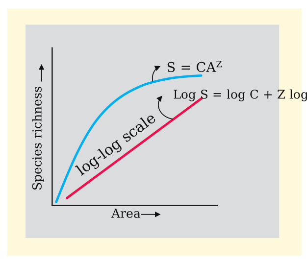
Drawn by us to help you understand the concept clearly, and verified to make sure it's accurate. For exams, practice from your textbook's own diagram.
The figure plots one single set of axes — species richness (S) on the vertical axis against area explored (A) on the horizontal — and draws two curves superimposed in that same box, not two separate panels.
The blue curve is the raw relationship, S = C x A^Z: a rectangular hyperbola that rises steeply from the origin, then gradually flattens as area keeps increasing. A small patch of new habitat initially yields many new species, but beyond a point even large expansions add very few.
The red line, labelled "log-log scale" and annotated log S = log C + Z log A, is the SAME relationship redrawn as a straight line — the figure's key point is that taking logs turns the hyperbola into a straight line, even though both curves are drawn together on the one plain (non-log-labelled) set of axes. …