Mathematics · Ch 10 — Vector Algebra
Some Basic Concepts
Some Basic Concepts
10.2 Some Basic Concepts
Directed Lines and Directed Line Segments
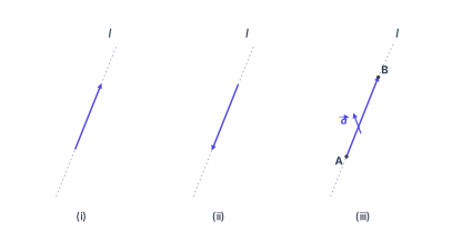
Consider any straight line in a plane or in three-dimensional space. This line can be traversed in two opposite directions, indicated by arrowheads. When we prescribe one of these two directions, the line becomes a directed line.
Now restrict the line to the segment between two points and . On this segment we have a definite length (the distance ) and one of the two possible directions. This gives a directed line segment.
A directed line segment has both magnitude (its length) and direction. This is the geometric representation of a vector.
Definition of a Vector
A vector is a quantity that has both magnitude and direction.
A directed line segment represents a vector. If the segment starts at point and ends at point , we denote the vector as or simply .
- Initial point: where the vector starts (point in ).
- Terminal point: where the vector ends (point in ).
- Magnitude (or length): the distance between the initial and terminal points. Denoted , , or simply .
- Direction: indicated by the arrowhead.
Since length is never negative, the notation has no meaning. Magnitude is always non-negative.
Position Vector
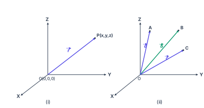
Recall the three-dimensional right-handed rectangular coordinate system from Class XI. Let be the origin and a point with coordinates .
The vector with as initial point and as terminal point is called the position vector of with respect to the origin, denoted or . By the distance formula:
The position vectors of points , , , etc., are usually denoted , , , respectively.
Direction Cosines
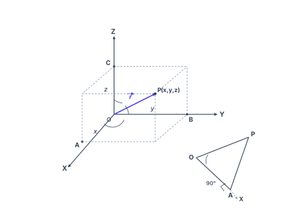
Consider the position vector of a point . Let , , be the angles that makes with the positive , , and -axes. These are the direction angles of the vector.
Their cosines — , , — are the direction cosines of , usually denoted , , . From the right-angled triangles formed by dropping perpendiculars from to each axis:
…
Definition
A vector is a quantity that has both magnitude and direction.
A directed line segment is a vector.
- It is denoted as or simply , and read as "vector " or "vector ".
- The point where the vector starts is called the initial point.
- The point where it ends is called the terminal point.
- The magnitude (or length) of the vector is the distance between its initial and terminal points, denoted as , , or .
- The arrow indicates the direction of the vector.
Note: Since length is never negative, the notation has no meaning.
Intuition
Think of a vector as an arrow — it tells you how far to go (magnitude) and which way to go (direction). A plain number (like 5 kg) has only magnitude; a vector (like "5 km east") has both.
Example …
Drawn by us to help you understand the concept clearly, and verified to make sure it's accurate. For exams, practice from your textbook's own diagram.
Fig 10.1 is a three‑panel diagram that builds the idea of a vector from the most basic geometric object: a straight line.
Panel (i) shows a straight line l drawn as a dotted line. A solid arrow runs upward along it. This arrow gives the line a direction — one of the two possible ways to travel along l. The line together with this chosen direction is called a directed line.
Panel (ii) shows the same dotted line l, but now the solid arrow points downward. This is the opposite direction. The two panels together make the point: any straight line can be given two directions, and a directed line is simply a line with one of those directions prescribed.
Panel (iii) is the crucial step. Instead of the whole infinite line, we now restrict ourselves to the line segment from point to point . The segment is drawn as a solid arrow from to , and the vector is labelled (or ). This is a directed line segment — it has a definite length (the distance ) and a definite direction (from to ). The textbook then defines a vector as exactly this: a quantity that has both magnitude and direction.
The point is called the initial point (or tail) and is the terminal point (or head). The magnitude of the vector is written , , or simply , and it is always non‑negative. The notation has no meaning.
The figure does not show any axes or coordinates — it is purely geometric. Its purpose is to separate the concept of direction (panels i and ii) from the concept of a vector as a directed segment with a specific length (panel iii). Once this foundation is laid, the textbook moves to the coordinate system and introduces the position vector of a point relative to the origin :
with magnitude
From there, the direction cosines are defined. If are the angles that makes with the positive , , and axes respectively, then
…
Drawn by us to help you understand the concept clearly, and verified to make sure it's accurate. For exams, practice from your textbook's own diagram.
Fig 10.2 is the textbook’s first visual bridge between the coordinate geometry you studied in Class XI and the vector language of Class XII. It shows two related 3‑D sketches, both drawn in a right‑handed coordinate system with the Z‑axis pointing straight up, the Y‑axis to the right, and the X‑axis coming toward the lower left. The origin is labelled O.
Panel (i) — the left sketch — introduces the position vector. A point is placed somewhere in the first octant (all coordinates positive). A solid arrow, usually coloured indigo in the printed book, runs from O to P. This arrow is the vector . Its length is the distance from the origin to P, which by the distance formula is
The dashed lines from P back to the axes (dropping perpendiculars to the coordinate planes) make it clear that , , are the components of along the three axes. So the figure’s first message is: every point in space corresponds to a unique position vector from the origin, and the coordinates of the point are exactly the components of that vector.
Panel (ii) — the right sketch — generalises the idea. Now three different points , , are shown, each with its own position vector from O: , , . All three vectors are coinitial — they share the same starting point O. This panel prepares you for the notation used throughout the chapter: the position vector of any point is written as (or ). It also sets up the visual habit of thinking of vectors as arrows radiating from a common origin, which is essential when you later add vectors or resolve them into components.
The position vector of a point is the vector from the origin to . Its magnitude is
The coordinates are the scalar components of along the , , axes.
The textbook uses this figure to lead directly into the definition of direction cosines (Fig 10.3, which follows immediately). In that next figure, the same position vector is shown with the angles , , that it makes with the positive , , axes. From the right‑angled triangles visible in the sketch — triangle in the ‑plane, in the ‑plane, and in the ‑plane — you get
where . These three cosines are called the direction cosines of the vector, and they satisfy . The coordinates can then be written as , which is a compact way of saying that the vector’s direction is completely specified by its direction cosines, and its length scales them. …
Drawn by us to help you understand the concept clearly, and verified to make sure it's accurate. For exams, practice from your textbook's own diagram.
Fig 10.3 is the central diagram for understanding how a vector in 3D space is described by its components and its direction. It shows a point in the first octant of a right-handed rectangular coordinate system, with the origin at the corner of a dashed rectangular box (a cuboid) whose edges lie along the positive , , and axes.
The position vector is drawn as a solid arrow (indigo in the original) from to , cutting diagonally through the interior of the cuboid. The three edges of the cuboid that meet at are the coordinate axes; the three edges that meet at are parallel to the axes. The projections of onto the axes are labelled (on the -axis), (on the -axis), and (on the -axis). The lengths , , and are exactly the coordinates , , and of , respectively. So the dashed cuboid makes it visually clear that to go from to you can travel units along , then units parallel to , then units parallel to — or take the direct vector .
At the origin , three small arcs indicate the direction angles , , and that makes with the positive , , and axes. These are the angles between the vector and each axis, measured in the usual way (between and ).
The figure also isolates a right triangle , with the right angle at (where the perpendicular from meets the -axis). In this triangle, is the adjacent side to angle , is the hypotenuse, and is the opposite side. From this triangle the textbook derives the first direction cosine:
Similarly, by considering the right triangles (right angle at ) and (right angle at ), you get:
These three cosines are called the direction cosines of , often denoted by , , and respectively. The magnitude is given by the distance formula:
where .
Because , , , the coordinates of can be written as where , , . The numbers , , are called the direction ratios of , often denoted by , , .
The direction cosines always satisfy , but in general (since , etc., and is not necessarily 1). …