Physics · Ch 11 — Dual Nature of Radiation and Matter
Effect of Frequency of Incident Radiation on Stopping Potential
Effect of Frequency of Incident Radiation on Stopping Potential
The Core Question: Does the Colour of Light Matter?
The previous experiments held the light's frequency constant and varied its intensity. Now we ask a different question: if we keep the intensity the same but change the frequency (the colour) of the light, what happens to the photoelectrons? The answer reveals the most important clue to the particle nature of light.
The Experiment: Varying Frequency at Fixed Intensity
We set up the same photoelectric effect apparatus. This time, we carefully adjust the light source so that the intensity (energy per second per unit area) is the same for every frequency we test. We then measure the photocurrent as a function of the collector plate potential for several different frequencies, say , , and , where .
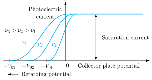
The results are shown in Figure 11.4 of the textbook. The key observations are:
-
Same Saturation Current: For all three frequencies, the saturation current is identical. This makes sense because the saturation current depends only on the number of photoelectrons emitted per second, which is determined by the intensity of the light. Since we kept the intensity constant, the number of emitted electrons is the same, and so is the saturation current.
-
Different Stopping Potentials: The stopping potential is not the same. It is different for each frequency. Specifically, the stopping potential is more negative for higher frequencies. The graph shows , corresponding to .
The stopping potential depends on the frequency of the incident radiation, not on its intensity. A higher frequency requires a larger retarding potential to stop the most energetic photoelectrons.
The Linear Relationship: Stopping Potential vs. Frequency
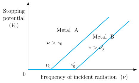
If we take the data from Figure 11.4 and plot the stopping potential (on the y-axis) against the frequency (on the x-axis) for a given photosensitive material, we get a straight line. This is shown in Figure 11.5 of the textbook. This single graph contains two profound results.
Property (i): Linear Variation
The stopping potential varies linearly with the frequency of the incident radiation for a given photosensitive material. The graph is a straight line with a positive slope.
Since the maximum kinetic energy of a photoelectron is , this immediately implies that also varies linearly with .
Property (ii): The Threshold Frequency
The straight line does not pass through the origin. It intercepts the frequency axis at a specific point, . At this frequency, the stopping potential is zero (). This means that for incident light of frequency , the most energetic photoelectrons are ejected with zero kinetic energy — they can just barely escape the metal surface.
This minimum frequency is called the threshold frequency. For any frequency , the stopping potential would be positive (meaning we would need to accelerate the electrons to get any current), which is impossible. Therefore, no photoelectric emission occurs at all, no matter how intense the light is.
The threshold frequency is a property of the metal, not the light. Different metals have different threshold frequencies. For example, selenium has a lower threshold frequency than zinc, which is why it is more sensitive to visible light. Copper has a high threshold frequency, so only ultraviolet light can cause the photoelectric effect in copper; green or red light cannot.
The Two Major Implications
The straight-line graph in Figure 11.5 leads to two fundamental conclusions about the photoelectric effect:
-
Kinetic Energy Depends on Frequency, Not Intensity: The maximum kinetic energy of the photoelectrons, , varies linearly with the frequency of the incident radiation. It is completely independent of the light's intensity. This directly contradicts the classical wave theory, which predicted that a more intense wave (with more energy) would always give the electrons more kinetic energy.
-
The Existence of a Threshold: For a frequency lower than the threshold frequency , no photoelectric emission is possible, even if the intensity is enormous. This is another direct contradiction of wave theory, which predicted that given enough time, even a weak wave of any frequency could transfer enough energy to an electron to eject it.
The Instantaneous Nature of Emission
A final, crucial experimental observation is the instantaneous nature of the effect. In all experiments, if the frequency of the incident radiation exceeds the threshold frequency, photoelectric emission starts without any measurable time lag, even when the incident radiation is extremely dim. It is now known that this emission begins in a time of the order of s or less.
This instantaneous start is a devastating blow to the classical wave theory. According to that theory, the energy of a light wave is spread uniformly over its wavefront. A single electron would need to collect energy from a large area over a significant amount of time before it had enough to escape. For very dim light, this "energy collection time" should be minutes or hours. The fact that emission is instantaneous shows that energy is not being collected gradually; it is being delivered in discrete packets.
Summary of Experimental Features …
Drawn by us to help you understand the concept clearly, and verified to make sure it's accurate. For exams, practice from your textbook's own diagram.
Fig. 11.4 is a graph of photoelectric current (vertical axis) against collector plate potential (horizontal axis). The horizontal axis is marked with negative (retarding) potentials to the left of the origin and positive (accelerating) potentials to the right. Three separate curves are drawn, one for each of three frequencies , all at the same intensity of incident light.
On the right side of the graph, all three curves rise to exactly the same saturation current. This tells you that the total number of photoelectrons emitted per second is the same for all three frequencies — because the intensity (number of photons per second) is kept fixed. On the left side, each curve cuts the horizontal axis at a different negative potential: (most negative) for , then , then (closest to the origin) for . These are the stopping potentials. The higher the frequency, the more negative the stopping potential.
The physical idea is straightforward. The stopping potential is the retarding voltage that just barely stops the fastest photoelectrons from reaching the collector. A more negative means those electrons had a larger maximum kinetic energy when they left the metal. So the graph shows that higher-frequency light gives photoelectrons more kinetic energy, even though the light intensity (and therefore the number of electrons) is unchanged.
From this figure, the textbook develops the central linear relation between stopping potential and frequency. For a given photosensitive material, the stopping potential varies linearly with the frequency of the incident radiation:
Here is Planck's constant, is the magnitude of the electron charge, and is the threshold frequency — the minimum frequency below which no photoelectrons are emitted, no matter how intense the light. The maximum kinetic energy of the emitted photoelectrons is , so the same relation can be written as:
This is Einstein's photoelectric equation. The figure directly demonstrates that depends only on frequency, not on intensity — because the three curves have the same saturation current (same number of electrons) but different stopping potentials (different maximum energies). The threshold frequency is the intercept on the frequency axis when ; for frequencies below , the stopping potential would be negative of a positive number that doesn't exist — meaning no emission occurs. …
Drawn by us to help you understand the concept clearly, and verified to make sure it's accurate. For exams, practice from your textbook's own diagram.
Fig. 11.5 is a graph that captures the most important quantitative relationship in the photoelectric effect. The horizontal axis is the frequency of the incident light. The vertical axis is the stopping potential , which is the retarding voltage needed to just stop the most energetic photoelectrons from reaching the collector.
For a given photosensitive material, the data points fall on a straight line. The line does not start at the origin. It meets the frequency axis at a positive value labelled , the threshold frequency for that material. To the left of , no photoelectrons are emitted at all, so there is no data and no line. The line itself has a positive slope, and the textbook explicitly annotates that slope as , where is Planck's constant and is the elementary charge.
The figure actually shows two such straight lines, one for metal A and one for metal B. Both lines have exactly the same slope — they are parallel. The only difference is where each line cuts the frequency axis. The metal with the higher work function has its threshold frequency further to the right. This is a direct visual demonstration that the threshold frequency is a material property, while the slope of the vs graph is a universal constant.
The physical idea is straightforward: the stopping potential measures the maximum kinetic energy of the photoelectrons, because . The graph shows that increases linearly with frequency, not with intensity. The line's equation, read directly from the graph, is the Einstein photoelectric equation in its most useful form:
or equivalently
Here is the charge of the electron ( C), is Planck's constant ( J s), is the frequency of the incident light, and is the threshold frequency for that metal. The term is the work function of the metal — the minimum energy needed to free an electron from its surface.
A common mistake is to think the slope of the vs graph is . It is not. The slope is , because the vertical axis is stopping potential (voltage), not energy. To get from the graph, you must multiply the slope by . …