Physics · Ch 1 — Electric Charges and Fields

The Field of an Electric Dipole

1.10.1

The Field of an Electric Dipole

Concept: The Electric Field of a Dipole

An electric dipole consists of two equal and opposite charges, $+q$ and $-q$ , separated by a small distance $2a$ . The electric field at any point in space is found by applying Coulomb’s law for each charge and then using the superposition principle (vector addition of fields). The field is simplest to calculate in two special directions: along the dipole axis and in the equatorial plane.

1. Field on the Dipole Axis (End-on Position)

Consider a point $P$ on the axis of the dipole, at a distance $r$ from the centre of the dipole, on the side of the $+q$ charge. The unit vector $\hat{\mathbf{p}}$ points from $-q$ to $+q$ (along the dipole axis).

Field due to $+q$ (at distance $r-a$ from $P$ ):

\mathbf{E}_{+q} = \frac{1}{4\pi\varepsilon_0} \frac{q}{(r-a)^2} \hat{\mathbf{p}}

Field due to $-q$ (at distance $r+a$ from $P$ ):

\mathbf{E}_{-q} = -\frac{1}{4\pi\varepsilon_0} \frac{q}{(r+a)^2} \hat{\mathbf{p}}

(The negative sign indicates the field points opposite to $\hat{\mathbf{p}}$ because $-q$ attracts a positive test charge.)

Total field (by superposition):

\mathbf{E} = \mathbf{E}_{+q} + \mathbf{E}_{-q} = \frac{q}{4\pi\varepsilon_0} \left[ \frac{1}{(r-a)^2} - \frac{1}{(r+a)^2} \right] \hat{\mathbf{p}}

Simplifying the bracket:

\mathbf{E} = \frac{q}{4\pi\varepsilon_0} \frac{4ar}{(r^2 - a^2)^2} \hat{\mathbf{p}}

For large distances ( $r \gg a$ ), we neglect $a^2$ compared to $r^2$ :

\mathbf{E} = \frac{2qa}{4\pi\varepsilon_0 r^3} \hat{\mathbf{p}} = \frac{2p}{4\pi\varepsilon_0 r^3} \hat{\mathbf{p}} \quad (r \gg a)

where $p = q \times 2a$ is the dipole moment.

2. Field on the Equatorial Plane

The equatorial plane is the plane perpendicular to the dipole axis and passing through its centre. For a point $P$ on this plane at distance $r$ from the centre:

The distances from $P$ to $+q$ and $-q$ are equal: $\sqrt{r^2 + a^2}$ .
The magnitudes of the fields are equal:

|\mathbf{E}_{+q}| = |\mathbf{E}_{-q}| = \frac{1}{4\pi\varepsilon_0} \frac{q}{r^2 + a^2}

Direction: The fields are symmetric. Their components perpendicular to the dipole axis cancel. The components along the axis (opposite to $\hat{\mathbf{p}}$ ) add up. The angle $\theta$ between the field direction and the axis satisfies $\cos\theta = \frac{a}{\sqrt{r^2 + a^2}}$ .
Total field (opposite to $\hat{\mathbf{p}}$ ):

\mathbf{E} = - \left( 2 \times \frac{1}{4\pi\varepsilon_0} \frac{q}{r^2 + a^2} \times \frac{a}{\sqrt{r^2 + a^2}} \right) \hat{\mathbf{p}}

\mathbf{E} = - \frac{2qa}{4\pi\varepsilon_0 (r^2 + a^2)^{3/2}} \hat{\mathbf{p}}

For large distances ( $r \gg a$ ):

\mathbf{E} = - \frac{2qa}{4\pi\varepsilon_0 r^3} \hat{\mathbf{p}} = - \frac{p}{4\pi\varepsilon_0 r^3} \hat{\mathbf{p}} \quad (r \gg a)

3. Dipole Moment and General Behaviour

Definition of dipole moment: $\mathbf{p} = q \times 2a \, \hat{\mathbf{p}}$ …

Figure 1.17Electric field of a dipole at (a) a point on the axis, (b) a point on the equatorial plane of the dipole.

Fig. 1.17 — Electric field of a dipole at (a) a point on the axis, (b) a point on the equatorial plane of the dipole.

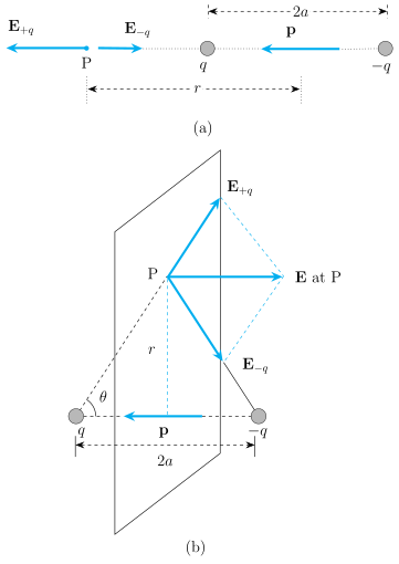
Drawn by us to help you understand the concept clearly, and verified to make sure it's accurate. For exams, practice from your textbook's own diagram.

What the Figure Shows

The figure has two stacked panels, (a) and (b), each depicting an electric dipole: two charges $+q$ and $-q$ separated by a distance $2a$ . The dipole moment vector $\mathbf{p}$ points from $-q$ to $+q$ along the axis. Panel (a) shows a point $P$ on the dipole axis, to the right of $+q$ . Panel (b) shows a point $P$ on the equatorial plane — the plane perpendicular to the dipole axis through its midpoint — located directly above the centre.

Physical Idea Illustrated

The figure teaches how the electric field of a dipole is obtained by vector addition of the fields due to each charge, using the superposition principle. The two special cases — axial and equatorial — are chosen because the symmetry simplifies the result.

On the axis (panel a): Both $\mathbf{E}_{+q}$ and $\mathbf{E}_{-q}$ point along the axis. Since $P$ is closer to $+q$ , $\mathbf{E}_{+q}$ is stronger than $\mathbf{E}_{-q}$ , and they partially cancel. The resultant $\mathbf{E}$ points away from $+q$ (same direction as $\mathbf{p}$ ).
On the equatorial plane (panel b): The distances from $P$ to $+q$ and $-q$ are equal, so the magnitudes $E_{+q} = E_{-q}$ . Their directions are symmetric: each makes an angle $\theta$ with the axis. The components perpendicular to the axis cancel, while the components along the axis add. The resultant $\mathbf{E}$ points opposite to $\mathbf{p}$ (i.e., toward $-q$ ).

Key Formulas Developed from the Figure

For a dipole with charge $q$ , separation $2a$ , and dipole moment $\mathbf{p} = q \cdot 2a \, \hat{\mathbf{p}}$ (where $\hat{\mathbf{p}}$ is the unit vector from $-q$ to $+q$ ):

On the axis (point at distance $r$ from centre, $r \gg a$ ):

\mathbf{E} = \frac{2}{4\pi\varepsilon_0} \frac{\mathbf{p}}{r^3} \quad \text{(direction along } \hat{\mathbf{p}}\text{)}

On the equatorial plane (point at distance $r$ from centre, $r \gg a$ ): …

Start your 14-day free trial to unlock the full solution →

← Previous · 1.10Electric Dipole Next · 1.10.2 →Physical Significance of Dipoles