Domain and Range of Trigonometric Functions

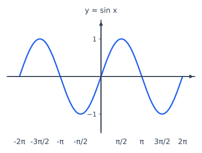
Fig. 3.8 is the graph of $y = \sin x$, plotted for $x$ from $-4\pi$ to $4\pi$. The horizontal axis is labelled $x$ and is marked at integer multiples of $\pi$: $\dots, -2\pi, -\pi, 0, \pi, 2\pi, \dots$. The vertical axis is labelled $y$ and runs from slightly below $-1$ to slightly above $1$, with dashed horizontal guide lines at $y = 1$ and $y = -1$ to show the amplitude.

The curve itself is a smooth, continuous wave that passes through the origin $(0,0)$. It rises from $0$ at $x=0$ to a maximum of $1$ at $x = \pi/2$, then falls back through $0$ at $x = \pi$ to a minimum of $-1$ at $x = 3\pi/2$, and returns to $0$ at $x = 2\pi$. This one complete up-and-down cycle — from $0$ to $1$ to $0$ to $-1$ and back to $0$ — is the fundamental shape of the sine function over an interval of length $2\pi$. The graph then repeats this exact pattern to the left and right, because $\sin x$ is periodic with period $2\pi$.

The physical idea the figure teaches is that $\sin x$ is bounded between $-1$ and $1$ for all real $x$, and that its values oscillate smoothly and predictably. The dashed lines at $y = \pm 1$ make the range $[-1, 1]$ visually immediate. The tick marks at multiples of $\pi$ help you see where the function crosses zero (at every integer multiple of $\pi$) and where it hits its extreme values (at odd multiples of $\pi/2$).

The key formula the textbook develops with this figure is the definition of the sine function itself, along with its domain (all real numbers) and range ($[-1, 1]$). The graph also directly supports the textbook's description of how $\sin x$ behaves in each quadrant: increasing from $0$ to $1$ in the first quadrant, decreasing from $1$ to $0$ in the second, decreasing from $0$ to $-1$ in the third, and increasing from $-1$ to $0$ in the fourth. You can trace this behaviour on the curve between $x = 0$ and $x = 2\pi$.

What Fig. 3.9 Shows

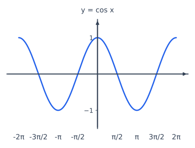
The graph of $y = \cos x$ is drawn for $x$ from $-4\pi$ to $4\pi$ — that is, two full cycles in each direction from the origin. The horizontal axis is marked at multiples of $\pi$: $\dots, -3\pi, -2\pi, -\pi, 0, \pi, 2\pi, 3\pi, 4\pi$. Two dashed horizontal lines are drawn at $y = 1$ and $y = -1$, showing the maximum and minimum values the cosine function ever attains. The curve itself begins at the point $(0, 1)$ and then oscillates smoothly between these two bounds. The label "$y = \cos x$" is placed directly on the curve.

What the Curve Teaches

The cosine wave is the most familiar periodic shape in mathematics — it repeats every $2\pi$ units. Starting at its maximum value $1$ when $x = 0$, it falls to $0$ at $x = \pi/2$, reaches its minimum $-1$ at $x = \pi$, returns to $0$ at $x = 3\pi/2$, and completes one full cycle back to $1$ at $x = 2\pi$. The same pattern repeats for negative $x$: because $\cos(-x) = \cos x$, the graph is symmetric about the $y$-axis.

The dashed lines at $y = \pm 1$ are not just decoration — they mark the range of the function. No matter what $x$ you plug in, $\cos x$ never goes above $1$ or below $-1$. This is the single most important numerical fact about cosine.

The Key Formula This Figure Supports

The textbook uses this graph to illustrate the domain and range of the cosine function:

Here $\mathbb{R}$ means "all real numbers" — you can take the cosine of any real number, no matter how large or small. The interval $[-1, 1]$ means every output lies between $-1$ and $1$, inclusive. The graph makes this concrete: the curve never leaves the horizontal strip between the two dashed lines.

How the Graph Connects to the Table of Behaviour

The textbook's table describes how $\cos x$ changes in each quadrant. You can see this directly on the graph:

• First quadrant ($0$ to $\pi/2$): the curve falls from $1$ to $0$ — cosine decreases.
• Second quadrant ($\pi/2$ to $\pi$): it continues falling from $0$ to $-1$ — still decreasing.
• Third quadrant ($\pi$ to $3\pi/2$): the curve rises from $-1$ to $0$ — cosine increases.
• Fourth quadrant ($3\pi/2$ to $2\pi$): it rises from $0$ to $1$ — still increasing. …

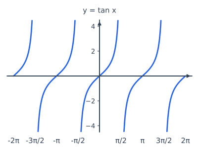
The graph of $y = \tan x$ shown in Fig. 3.10 covers the interval $x \in [-\pi, 2\pi]$. The horizontal axis is marked with ticks at $-\pi$, $-\pi/2$, $\pi/2$, $\pi$, $3\pi/2$, and $2\pi$. The vertical axis is not labelled with specific numbers, but the curve itself tells the story.

The most striking feature is the set of dashed vertical lines at $x = -\pi/2$, $x = \pi/2$, and $x = 3\pi/2$. These are asymptotes — the graph never touches or crosses them. Between each pair of consecutive asymptotes, the curve forms a single, continuous branch that rises from the bottom left to the top right. On the interval $(-\pi/2, \pi/2)$, the branch passes through the origin $(0,0)$ and increases smoothly. On $(\pi/2, 3\pi/2)$, another identical branch appears, shifted one period to the right. The pattern repeats: a third branch on $(3\pi/2, 5\pi/2)$ would continue beyond the drawn window, but the figure stops at $2\pi$, showing only the start of that branch.

What the graph teaches is that $\tan x$ is periodic with period $\pi$, not $2\pi$ like sine and cosine. The function is undefined at every odd multiple of $\pi/2$, where the asymptotes stand. As $x$ approaches an asymptote from the left, $\tan x$ shoots upward toward $+\infty$; from the right, it plunges downward toward $-\infty$. This behaviour matches the textbook's table: in the first quadrant ($0 < x < \pi/2$), $\tan x$ increases from $0$ to $\infty$, and in the second quadrant ($\pi/2 < x < \pi$), it increases from $-\infty$ to $0$.

The key formula that explains this periodicity is

which the textbook derives in the next section. Because $\tan x$ repeats every $\pi$ units, the graph's shape on $(-\pi/2, \pi/2)$ is identical to its shape on $(\pi/2, 3\pi/2)$, and so on. The domain is all real numbers except $x = (2n+1)\pi/2$, and the range is all real numbers — the graph covers every $y$-value, from $-\infty$ to $\infty$, across its branches.

What Fig. 3.11 Shows: The Graph of $y = \cot x$

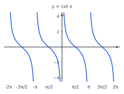
The figure plots the cotangent function over the interval $[-\pi, 2\pi]$ on the $x$-axis. The $y$-axis is unmarked but clearly extends to large positive and negative values. The curve consists of three separate, downward-sloping branches, each confined between a pair of dashed vertical lines. These dashed lines are the asymptotes — the $x$-values where $\cot x$ is undefined — located at $x = -\pi$, $x = 0$, $x = \pi$, and $x = 2\pi$.

Each branch of the curve falls continuously from the top-left to the bottom-right of its interval. Between $-\pi$ and $0$, the curve starts near $+\infty$ just to the right of $-\pi$, decreases smoothly, and plunges toward $-\infty$ as it approaches $0$ from the left. The same shape repeats between $0$ and $\pi$, and again between $\pi$ and $2\pi$. The curve never touches or crosses the asymptotes. The label "$y = \cot x$" is placed near one of the branches.

The Physical Idea: Reciprocal of Tangent, with Its Own Rhythm

The core idea is that $\cot x$ is the reciprocal of $\tan x$:

Because $\tan x$ is undefined at $x = \frac{\pi}{2} + n\pi$, its reciprocal $\cot x$ is zero at those points. Conversely, $\cot x$ is undefined wherever $\sin x = 0$ — that is, at $x = n\pi$ — because division by zero is impossible. This is why the asymptotes fall at integer multiples of $\pi$, not at the half-integer multiples where $\tan x$ has its asymptotes.

The graph's decreasing shape in each interval is not arbitrary. From the textbook's table, in the first quadrant ($0 < x < \frac{\pi}{2}$), $\cot x$ decreases from $\infty$ to $0$. In the second quadrant ($\frac{\pi}{2} < x < \pi$), it decreases from $0$ to $-\infty$. This pattern — decreasing from $+\infty$ to $-\infty$ across each interval of length $\pi$ — is the signature behaviour of the cotangent function.

Domain, Range, and Period — The Key Facts

The figure makes three essential properties visually obvious:

Domain: All real numbers except where $\sin x = 0$, i.e., $x \neq n\pi$ for any integer $n$. The asymptotes mark these excluded points.

Range: All real numbers ($-\infty < y < \infty$). Unlike sine and cosine, which are bounded between $-1$ and $1$, $\cot x$ can take any real value. The graph shoots up to $+\infty$ on one side of each asymptote and down to $-\infty$ on the other, covering every $y$-value in between.

Period: $\pi$. The pattern from $-\pi$ to $0$ repeats exactly from $0$ to $\pi$, and again from $\pi$ to $2\pi$. This is half the period of sine and cosine, which repeat every $2\pi$. The textbook notes this explicitly: since $\tan(\pi + x) = \tan x$, its reciprocal $\cot x$ also repeats after $\pi$.

How the Graph Connects to the Table of Behaviour …

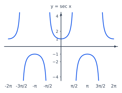
What Fig. 3.12 Shows

The graph of $y = \sec x$ is plotted for $x$ from $-\pi$ to $2\pi$ on the horizontal axis, with $y$ on the vertical axis. The curve consists of three distinct U-shaped branches, each opening either upward or downward, separated by vertical dashed lines called asymptotes.

The asymptotes occur at $x = -\frac{\pi}{2}$, $x = \frac{\pi}{2}$, and $x = \frac{3\pi}{2}$ — these are the points where $\cos x = 0$, and since $\sec x = \frac{1}{\cos x}$, the function is undefined there. The curve approaches these vertical lines but never touches them; as $x$ gets closer to an asymptote, $|y|$ grows without bound.

The central branch, around $x = 0$, opens upward like a U. Its lowest point is at $y = 1$ when $x = 0$ (since $\sec 0 = 1$). This branch lies entirely above $y = 1$, never dipping below. The branch around $x = \pi$ opens downward like an inverted U, with its highest point at $y = -1$ when $x = \pi$ (since $\sec \pi = -1$). This branch stays entirely below $y = -1$. The remaining branches at the edges of the plotted interval behave similarly — one upward branch near $x = -\pi$ and another near $x = 2\pi$, each approaching the asymptotes at the boundaries.

The axes are labelled, and the curve itself is labelled "$y = \sec x$".

The Physical Idea

The secant graph teaches you that $\sec x$ is the reciprocal of $\cos x$, so wherever $\cos x$ is zero, $\sec x$ blows up to infinity (positive or negative). Where $\cos x$ reaches its maximum of $1$, $\sec x$ hits its minimum of $1$; where $\cos x$ reaches its minimum of $-1$, $\sec x$ hits its maximum of $-1$. The function never takes values between $-1$ and $1$ — that gap is forbidden because a reciprocal of a number between $-1$ and $1$ would have magnitude greater than $1$.

The graph also shows the periodic nature: the pattern of branches repeats every $2\pi$, because $\sec(x + 2\pi) = \sec x$.

Key Formula Illustrated by the Figure

The definition that generates the entire graph is:

Here:

• $x$ is the angle (in radians) measured from the positive $x$-axis.
• $\cos x$ is the cosine of that angle.
• $\sec x$ is the secant, defined as the reciprocal of $\cos x$. …

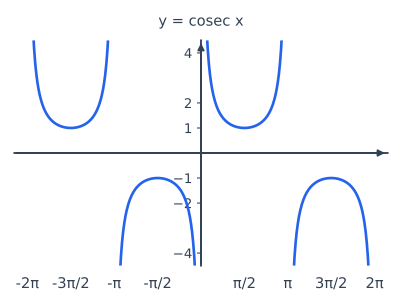
What Fig. 3.13 Shows: The Graph of $y = \csc x$

The figure plots the cosecant function over the interval $[-\pi, 2\pi]$, which is two full periods of the sine function (since $\csc x = 1/\sin x$ repeats every $2\pi$). The horizontal axis is labelled $x$ (in radians), and the vertical axis is $y$. Three key visual features stand out:

Asymptotes. Dashed vertical lines appear at $x = -\pi$, $x = 0$, $x = \pi$, and $x = 2\pi$. These are the points where $\sin x = 0$, so $\csc x = 1/0$ is undefined — the curve shoots off to $\pm\infty$ as it approaches these lines. The asymptotes divide the graph into three open intervals: $(-\pi, 0)$, $(0, \pi)$, and $(\pi, 2\pi)$.

The branches. On $(0, \pi)$, the curve forms an upward-opening U-shape. Its lowest point is at $y = 1$ (when $x = \pi/2$, where $\sin x = 1$). On $(-\pi, 0)$ and $(\pi, 2\pi)$, the branches are downward-opening inverted U-shapes, each reaching a maximum of $y = -1$ (at $x = -\pi/2$ and $x = 3\pi/2$, where $\sin x = -1$). The curve never lies between $-1$ and $1$ — it stays either above $1$ or below $-1$.

The label. The curve is clearly marked $y = \csc x$, and the axes are scaled so that the key points $(\pi/2, 1)$ and $(3\pi/2, -1)$ are visible.

The Physical Idea: Reciprocal Behaviour and Range

The figure teaches one central idea: the cosecant function exists only where its reciprocal, $\sin x$, is non-zero. Because $\csc x = 1/\sin x$, the graph is forced to "blow up" near the zeros of sine. This explains the domain and range given in the textbook:

The domain is all real $x$ except integer multiples of $\pi$: $\{x : x \in \mathbb{R}, x \neq n\pi, n \in \mathbb{Z}\}$. The range is $\{y : y \in \mathbb{R}, y \leq -1 \text{ or } y \geq 1\}$ — the graph never enters the strip $(-1, 1)$ because $|\sin x| \leq 1$ implies $|\csc x| \geq 1$.

Key Formula Developed with This Figure

The textbook uses the graph to reinforce the periodic nature and the sign pattern of $\csc x$ in each quadrant. The table in the textbook (reproduced in the grounding text) shows how $\csc x$ behaves: