Mathematics · Ch 5 — Continuity and Differentiability

Exponential and Logarithmic Functions

5.4

Exponential and Logarithmic Functions

5.4 Exponential and Logarithmic Functions

Why a New Class of Functions?

Polynomial functions grow at a rate set by their degree: for $x > 1$ , $f_n(x) = x^n$ rises faster as $n$ increases. This raises a question: is there a function that grows faster than any polynomial, no matter how high the degree?

The answer is yes. Take $f(x) = 10^x$ . At $x = 10^3$ , compare:

$f_{100}(x) = (10^3)^{100} = 10^{300}$
$f(x) = 10^{10^3} = 10^{1000}$

So $10^x$ dwarfs $x^{100}$ ; in fact $10^x > x^{100}$ for all $x > 10^3$ . More generally $b^x$ (with $b > 1$ ) outgrows any $x^n$ for large enough $x$ . This motivates the exponential functions.

The Exponential Function

b > 1

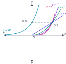
The graph of $y = 10^x$ is shown in Fig 5.9 of the textbook; sketching $y = 2^x$ , $y = 3^x$ , $y = 4^x$ shows how the base affects steepness.

Salient Features of Exponential Functions

Domain: all real numbers $\mathbb{R}$ .
Range: all positive reals $(0, \infty)$ .
Fixed point: $(0, 1)$ always lies on the graph, since $b^0 = 1$ .
Monotonicity: ever increasing — as $x$ increases, $b^x$ increases.
Large negative $x$ : $b^x$ is very close to $0$ ; the graph approaches the $x$ -axis (a horizontal asymptote) but never touches it.

Common and Natural Exponential Functions

When $b = 10$ , $y = 10^x$ is the common exponential function.
The special number $e$ is defined by

e = 1 + \frac{1}{1!} + \frac{1}{2!} + \frac{1}{3!} + \cdots

and lies between $2$ and $3$ . Base $e$ gives the natural exponential function $y = e^x$ .

The Logarithmic Function

The exponential function $b^x$ is one-to-one (strictly increasing), so it has an inverse — the logarithmic function.

b > 1

Examples

$2^3 = 8 \iff \log_2 8 = 3$ .
$10^4 = 10000 \iff \log_{10} 10000 = 4$ .
$625 = 5^4 = 25^2 \iff \log_5 625 = 4$ or $\log_{25} 625 = 2$ .

Logarithm as a Function

Fixing $b > 1$ , the logarithmic function is $\log_b : \mathbb{R}^+ \to \mathbb{R}$ , with $\log_b x = y$ if $b^y = x$ .

$b = 10$ : common logarithm.
$b = e$ : natural logarithm, denoted $\ln$ . In this chapter, $\log x$ means $\ln x$ (base $e$ ).

Important Observations About the Logarithm Function (any base $b > 1$ )

Domain: $\mathbb{R}^+$ ; the logarithm of a non-positive number is undefined.
Range: all real numbers $\mathbb{R}$ .
Fixed point: $(1, 0)$ always lies on the graph, since $\log_b 1 = 0$ .
Monotonicity: ever increasing — as $x$ increases, $\log_b x$ increases.
Near zero: for $x$ close to $0$ , $\log_b x$ can be made arbitrarily negative; the graph approaches the $y$ -axis (a vertical asymptote) but never touches it.
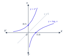
Mirror property: $y = e^x$ and $y = \ln x$ are mirror images in the line $y = x$ (Fig 5.11).

Properties of Logarithms (with Proofs)

Property 1: Change of Base Rule

\log_a p = \frac{\log_b p}{\log_b a}

›Proof

Proof: Let $\log_a p = \alpha$ , $\log_b p = \beta$ , $\log_b a = \gamma$ , so $a^\alpha = p$ , $b^\beta = p$ , $b^\gamma = a$ . Substituting $a = b^\gamma$ into $a^\alpha = p$ :

$(b^\gamma)^\alpha = b^{\gamma\alpha} = p = b^\beta$

Since the exponential is one-to-one, $\beta = \gamma\alpha$ , so $\alpha = \frac{\beta}{\gamma}$ , i.e.

$\log_a p = \frac{\log_b p}{\log_b a}$

Property 2: Product Rule

\log_b (pq) = \log_b p + \log_b q

›Proof

Proof: Let $\log_b(pq) = \alpha$ , $\log_b p = \beta$ , $\log_b q = \gamma$ , so $b^\alpha = pq$ , $b^\beta = p$ , $b^\gamma = q$ . Then

$b^\alpha = pq = b^\beta \cdot b^\gamma = b^{\beta + \gamma}$

so $\alpha = \beta + \gamma$ , that is $\log_b(pq) = \log_b p + \log_b q$ .

Special Case: Power Rule

With $p = q$ , the product rule gives $\log_b p^2 = 2\log_b p$ , and by repeated application (or induction), for any positive integer $n$ :

\log_b p^n = n \log_b p

Note

This result actually holds for any real number $n$ , not just positive integers, though that proof is beyond this text.

Property 3: Quotient Rule

\log_b \left(\frac{x}{y}\right) = \log_b x - \log_b y

›Proof

Proof: Let $\log_b\left(\frac{x}{y}\right) = \alpha$ , $\log_b x = \beta$ , $\log_b y = \gamma$ , so $b^\alpha = \frac{x}{y}$ , $b^\beta = x$ , $b^\gamma = y$ . Then

$b^\alpha = \frac{x}{y} = \frac{b^\beta}{b^\gamma} = b^{\beta - \gamma}$ …

Definition 3Exponential function

Exponential function

Fix a base $b > 1$ (a real number). The exponential function to base $b$ is the function

y = f(x) = b^{x}.

Here the exponent $x$ is the variable, and the base $b$ stays constant.

Domain and range:

The domain is all of $\mathbb{R}$ — you may raise $b$ to any real power.
The range is $(0,\infty)$ , so $b^{x} > 0$ for every $x$ .

The curve passes through $(0,1)$ (since $b^{0}=1$ ) and rises steadily as $x$ increases.

Concrete example: …

Definition 4Logarithm (logarithmic function to base b)

Definition of Logarithm

Let $b > 1$ be a fixed real number (the base).

For a positive real number $a$ , we say that the logarithm of $a$ to the base $b$ is $x$ if

b^x = a.

This is written as

\log_b a = x \quad \Longleftrightarrow \quad b^x = a.

Domain and range:

The logarithm $\log_b a$ is defined only for $a > 0$ (positive real numbers).
The value $x$ can be any real number.

Intuition:

A logarithm answers the question: "To what exponent must I raise the base $b$ to get $a$ ?" …

Theorem 5

Theorem 5 (Derivative of the Natural Exponential Function)

The derivative of $e^x$ with respect to $x$ is $e^x$ itself. That is,

\frac{d}{dx}(e^x) = e^x

This theorem holds for all real $x$ . No additional hypotheses are needed — the function $e^x$ is differentiable on its entire domain $\mathbb{R}$ .

Proof

›Proof

The proof uses the first principle of differentiation (the definition of the derivative):

$f'(x) = \lim_{h \to 0} \frac{f(x+h) - f(x)}{h}$

For $f(x) = e^x$ , we have:

$\frac{d}{dx}(e^x) = \lim_{h \to 0} \frac{e^{x+h} - e^x}{h}$

Step 1: Factor out $e^x$

Using the law of exponents $e^{x+h} = e^x \cdot e^h$ :

$\frac{d}{dx}(e^x) = \lim_{h \to 0} \frac{e^x \cdot e^h - e^x}{h} = \lim_{h \to 0} \frac{e^x(e^h - 1)}{h}$

Since $e^x$ does not depend on $h$ , it can be taken outside the limit:

$\frac{d}{dx}(e^x) = e^x \cdot \lim_{h \to 0} \frac{e^h - 1}{h}$

Step 2: Evaluate the limit $\displaystyle \lim_{h \to 0} \frac{e^h - 1}{h}$

Recall that $e$ is defined as:

$e = \lim_{n \to \infty} \left(1 + \frac{1}{n}\right)^n$

Equivalently, for small $h$ , we can write $e^h \approx 1 + h$ (this is the linear approximation of $e^h$ near $h=0$ ). More precisely, the limit:

$\lim_{h \to 0} \frac{e^h - 1}{h} = 1$

This is a standard limit whose proof relies on the series expansion of $e^h$ or on the definition of $e$ itself. The NCERT text states this result without deriving it here, as a rigorous proof is beyond the scope of this chapter.

Step 3: Conclude

Substituting the limit value:

$\frac{d}{dx}(e^x) = e^x \cdot 1 = e^x$

Hence, $\displaystyle \frac{d}{dx}(e^x) = e^x$ , as required.

When Is This Used?

This result is the foundation for differentiating any function involving $e^x$ , especially when combined with the chain rule. For example, to differentiate $e^{g(x)}$ , we use:

$\frac{d}{dx} e^{g(x)} = e^{g(x)} \cdot g'(x)$ …

Figure 5.9Graphs of the power functions y = x, y = x², y = x³, y = x⁴ together with the exponential y = 10ˣ, comparing their rates of growth

Fig. 5.9 — Graphs of the power functions y = x, y = x², y = x³, y = x⁴ together with the exponential y = 10ˣ, comparing their rates of growth

Drawn by us to help you understand the concept clearly, and verified to make sure it's accurate. For exams, practice from your textbook's own diagram.

Fig. 5.9 is a single plot with five curves, four of which pass through both the origin $(0,0)$ and the point $(1,1)$ ; the fifth (the exponential) passes through $(0,1)$ and $(1,1)$ -ish region but is drawn to a different, non-literal scale, as is typical in this schematic sketch. The horizontal axis is $x$ , the vertical axis is $y$ . The five functions drawn are:

$y = x$ — a straight line through the origin, shown as an indigo line, drawn only for $x \ge 0$ .
$y = x^2$ — drawn only for $x \ge 0$ here (the figure restricts every power-function curve to the positive $x$ -axis, fanning out from the origin).
$y = x^3$ — drawn only for $x \ge 0$ in this figure.
$y = x^4$ — the steepest of the four power curves for $x>1$ , also drawn only for $x \ge 0$ .
$y = 10^x$ — the steepest curve of all. Unlike the four power functions, it is drawn for negative $x$ too: it hugs the $x$ -axis closely (but never touches it) as $x \to -\infty$ , passes through $(0,1)$ , and then rises far more steeply than any of the power curves.

The points $(0,1)$ and $(1,1)$ are marked and joined by a dashed horizontal guide line. Each curve is labelled directly on the figure, in the order (steepest to least steep near $x=1$ ): $y=10^x$ , $y=x^4$ , $y=x^3$ , $y=x^2$ , $y=x$ .

The central idea the figure teaches is rate of growth. Among the four power functions, as the exponent $n$ increases from $1$ to $4$ , the curves become steeper for $x>1$ . For a fixed increment in $x$ (say from $1$ to $2$ ), the corresponding increment in $y$ grows dramatically with $n$ :

$x=1 \to 2$ : $y=x$ goes from $1$ to $2$ (increase of $1$ ).
$y=x^2$ goes from $1$ to $4$ (increase of $3$ ).
$y=x^3$ goes from $1$ to $8$ (increase of $7$ ).
$y=x^4$ goes from $1$ to $16$ (increase of $15$ ).

The textbook uses this visual to argue that higher-degree polynomial functions grow faster than lower-degree ones for $x>1$ , and then poses the question: is there a function that grows faster than any polynomial? The answer is the exponential function $y = 10^x$ , which for $x=10^3$ gives $10^{1000}$ — far larger than $x^{100} = 10^{300}$ . The figure itself draws this exponential curve alongside the power functions to make the comparison visually immediate, even though (being schematic) it is not drawn strictly to the same numeric scale as the power curves beyond $x \approx 1$ .

f_n(x) = x^n \quad (n = 1,2,3,4,\dots), \qquad f(x) = 10^x

Figure 5.10Graphs of y = log₂x, y = logₑx, and y = log₁₀x, showing how the base of a logarithm changes its rate of growth

Fig. 5.10 — Graphs of y = log₂x, y = logₑx, and y = log₁₀x, showing how the base of a logarithm changes its rate of growth

Drawn by us to help you understand the concept clearly, and verified to make sure it's accurate. For exams, practice from your textbook's own diagram.

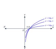
Fig 5.10 shows three logarithmic curves on the same set of axes: $y = \log_2 x$ , $y = \log_e x$ (often written as $y = \ln x$ ), and $y = \log_{10} x$ . The horizontal axis is the $x$ -axis (positive real numbers only, since logarithms are undefined for $x \le 0$ ), and the vertical axis is the $y$ -axis (all real numbers). Each curve passes through the point $(1,0)$ because $\log_b 1 = 0$ for any base $b > 1$ . The curves are ordered by their base: the curve for base 2 is the topmost, base $e$ is in the middle, and base 10 is the lowest. All three rise slowly as $x$ increases beyond 1, and as $x$ approaches 0 from the right, each curve drops steeply toward $-\infty$ , getting arbitrarily close to the $y$ -axis without ever touching it.

The central idea this figure teaches is that logarithmic functions with different bases are all increasing functions (for $b > 1$ ), but they grow at different rates. A larger base gives a slower rate of increase — that is why $\log_2 x$ lies above $\log_e x$ , which lies above $\log_{10} x$ , for any $x > 1$ . Conversely, for $0 < x < 1$ , the ordering reverses: the curve with the larger base is lower (more negative). The figure also illustrates the key properties listed in the textbook: the domain is $x > 0$ , the range is all real numbers, the point $(1,0)$ is always on the graph, and the function is ever-increasing.

The textbook uses this figure to introduce the logarithmic function and then develops two essential formulas. The first is the change-of-base rule:

\log_a p = \frac{\log_b p}{\log_b a}

Here $a$ and $b$ are any bases greater than 1, and $p > 0$ . This formula lets you convert a logarithm from one base to another — for instance, to compute $\log_2 5$ using natural logs: $\log_2 5 = \frac{\ln 5}{\ln 2}$ .

The second key result is the product rule for logarithms:

\log_b (pq) = \log_b p + \log_b q

where $b > 1$ , $p > 0$ , $q > 0$ . A direct consequence is the power rule: $\log_b (p^n) = n \log_b p$ for any real $n$ (the textbook proves it for positive integers and states it holds for all real $n$ ). There is also the quotient rule: $\log_b \left(\frac{x}{y}\right) = \log_b x - \log_b y$ . …

Figure 5.11Graphs of y = eˣ and y = logₑx as mirror images in y = x

Fig. 5.11 — Graphs of y = eˣ and y = logₑx as mirror images in y = x

Drawn by us to help you understand the concept clearly, and verified to make sure it's accurate. For exams, practice from your textbook's own diagram.

Fig. 5.11 is a single Cartesian plot with two curves and one dashed line. The horizontal axis is labelled $x$ , the vertical axis is labelled $y$ , and both axes are drawn to the same scale so that the line $y = x$ (dashed) runs at $45^\circ$ through the origin.

The first curve is $y = e^x$ . It passes through $(0,1)$ and rises steeply as $x$ increases. For negative $x$ , the curve hugs the $x$ -axis very closely but never touches it — this is the horizontal asymptote $y = 0$ . The second curve is $y = \log_e x$ (often written as $\ln x$ ). It passes through $(1,0)$ and rises slowly for $x > 1$ . As $x$ approaches $0$ from the right, the curve plunges downward without bound, approaching the $y$ -axis as a vertical asymptote. The two points $(0,1)$ and $(1,0)$ are marked explicitly. All three lines — $y = e^x$ , $y = x$ , and $y = \log_e x$ — are labelled directly on the figure.

The physical idea is that the exponential function and the natural logarithm are inverses of each other. When you reflect the graph of $y = e^x$ across the line $y = x$ , you obtain the graph of $y = \log_e x$ , and vice versa. This mirror-image relationship is the geometric signature of inverse functions: if a point $(a,b)$ lies on one curve, then $(b,a)$ lies on the other. Here, $(0,1)$ on $e^x$ reflects to $(1,0)$ on $\log_e x$ , exactly as expected.

Important

The figure visually confirms the inverse relationship:

$y = e^x \quad \Longleftrightarrow \quad x = \log_e y$

For every point $(x, e^x)$ on the exponential curve, the reflected point $(e^x, x)$ lies on the logarithmic curve.

The textbook uses this figure to anchor two fundamental derivative results, stated as Theorem 5:

\frac{d}{dx}(e^x) = e^x

Start your 14-day free trial to unlock the full solution →

← Previous · 5.3.3Q15 — Find (dy)/(dx) in the following: y = sec⁻¹ ((1)/(2x²-1)), 0 < x < frac…Next · 5.4 →Example 25 — Is it true that x = elog x for all real x?

Exponential and Logarithmic Functions