Physics · Ch 2 — Electrostatic Potential and Capacitance
Equipotential Surfaces
Equipotential Surfaces
What is an Equipotential Surface?
An equipotential surface is a surface over which the electric potential is constant at every point.
This means that the potential difference between any two points on the same equipotential surface is zero.
Why the Electric Field is Perpendicular to an Equipotential Surface
If the electric field had a component along the surface, then to move a unit positive test charge along that component, work would have to be done (since work = force × displacement).
But on an equipotential surface, no work is required to move a test charge between any two points (because ).
Therefore, the electric field cannot have a component parallel to the surface.
Hence, the electric field is always normal (perpendicular) to the equipotential surface at every point.
Equipotential Surfaces for a Single Point Charge
For a point charge , the potential at a distance is given by:
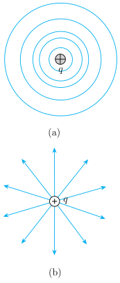
Since is constant when is constant, the equipotential surfaces are concentric spherical surfaces centred at the charge.
The electric field lines for a single point charge are radial lines (starting from the charge if , ending at the charge if ).
These radial field lines are normal to the spherical equipotential surfaces at every point.
Equipotential Surfaces for a Uniform Electric Field
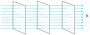
For a uniform electric field directed along the -axis, the potential changes only along .
Thus, surfaces of constant are planes perpendicular to the -axis — that is, planes parallel to the - plane.
Equipotential Surfaces for a Dipole and Two Identical Positive Charges …
Drawn by us to help you understand the concept clearly, and verified to make sure it's accurate. For exams, practice from your textbook's own diagram.
What the Figure Shows
The figure has two panels, (a) and (b), both centred on a single point charge labelled q (with a ⊕ symbol, indicating a positive charge).
-
Panel (a) shows five concentric circles around the charge. These circles represent equipotential surfaces — surfaces where the electric potential has the same value everywhere. The circles are drawn closer together near the charge, indicating that the potential changes more rapidly as you approach the charge.
-
Panel (b) shows eight straight arrows radiating outward from the charge in evenly spaced directions. These arrows represent electric field lines for a positive charge , which point radially outward.
Physical Idea Taught
The figure illustrates two complementary visual representations of the electric field around a single point charge:
-
Equipotential surfaces are spherical (concentric circles in 2D cross-section) because the potential depends only on the distance from the charge: . For a fixed , is constant, so each sphere of radius is an equipotential surface.
-
Electric field lines are radial, starting from the charge if (or ending at it if ). The field is always normal (perpendicular) to the equipotential surface at every point. This is a general principle: if the field had a component along the surface, work would be required to move a test charge on that surface, contradicting the definition of an equipotential surface (no work needed).
Key Formula
The potential due to a single point charge at a distance is:
- = electric potential (in volts)
- = magnitude of the point charge (in coulombs)
- = distance from the charge (in metres)
- = permittivity of free space () …
Drawn by us to help you understand the concept clearly, and verified to make sure it's accurate. For exams, practice from your textbook's own diagram.
What the figure shows
The diagram depicts three vertical, parallel planes drawn as tall parallelograms in oblique perspective. They are evenly spaced from left to right. A set of many parallel horizontal field lines runs through all three planes, with arrowheads pointing to the right. The bold label E is placed at the far right, beside the arrow tips. The planes are perpendicular to the field lines.
Physical idea
The figure illustrates that for a uniform electric field (constant in magnitude and direction), the equipotential surfaces are planes that are normal (perpendicular) to the field direction. In this case, the field is along the -axis, so the equipotential surfaces are planes parallel to the - plane. The spacing between the planes corresponds to a constant potential difference between them.
Key formula
The relationship between the uniform field and the potential difference between two equipotential surfaces separated by a perpendicular distance is:
where:
- is the potential difference between two equipotential surfaces (in volts, V)
- is the magnitude of the uniform electric field along the -axis (in volts per metre, V/m)
- is the perpendicular distance between the two surfaces (in metres, m) …
Drawn by us to help you understand the concept clearly, and verified to make sure it's accurate. For exams, practice from your textbook's own diagram.
What the Figure Shows
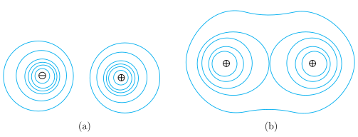
The figure has two side-by-side panels, (a) and (b), each showing equipotential surfaces (curves of constant electric potential) in a plane containing the charges.
-
Panel (a): A dipole
A negative charge () is at the upper left, and a positive charge () at the lower right. Around each charge, the equipotential surfaces are nearly circular close to the charge, but as you move away, the curves distort toward each other between the charges. This distortion reflects the combined potential of both charges.
-
Panel (b): Two identical positive charges
Two equal positive charges () are placed side by side. Near each charge, the equipotential surfaces are small concentric circles. Farther away, the surfaces merge into larger contours that enclose both charges, forming a peanut-shaped or figure-eight outer boundary. The region between the charges has a saddle point where the potential is locally flat.
Physical Idea
Equipotential surfaces are surfaces (here drawn as curves in a plane) where the electric potential is constant. The key property is that the electric field is always perpendicular to the equipotential surface at every point. This follows because moving a test charge along an equipotential requires no work — if had a component along the surface, work would be done, contradicting the definition.
The figure illustrates how equipotential surfaces change shape for different charge configurations:
- For a single point charge, they are concentric spheres (circles in a plane).
- For a dipole, the surfaces are distorted, showing the influence of both charges.
- For two like charges, the surfaces merge at large distances, reflecting the net repulsive field.
Key Formula
The potential due to a single point charge at a distance is:
where:
- = electric potential (in volts)
- = charge (in coulombs)
- = distance from the charge (in metres)
- = permittivity of free space ()
For a dipole (two charges and separated by distance ), the potential at a point far away (distance ) is:
…