Magnetic Field on the Axis of a Circular Current Loop

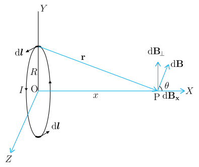
The figure shows a circular loop of radius $R$ lying in the Y–Z plane, with its centre at the origin $O$. The X-axis is the axis of the loop, pointing to the right. The loop carries a steady current $I$ (direction indicated by arrows on the loop). A point $P$ is marked on the X-axis at a distance $x$ from $O$.

Two specific current elements are highlighted:

• A line element $d\mathbf{l}$ at the top of the loop (in the Y–Z plane).
• Another $d\mathbf{l}$ diametrically opposite at the bottom of the loop.

From the top $d\mathbf{l}$, a displacement vector $\mathbf{r}$ (shown in blue) runs to point $P$. The magnitude of $\mathbf{r}$ is $r = \sqrt{x^2 + R^2}$.

At point $P$, the magnetic field $d\mathbf{B}$ due to the top $d\mathbf{l}$ is drawn perpendicular to $\mathbf{r}$ (as required by the Biot–Savart law). This $d\mathbf{B}$ is then resolved into two components:

• $dB_x$ — along the X-axis (to the right).
• $dB_\perp$ — perpendicular to the X-axis (vertical up).

The angle $\theta$ is marked at $P$ between $d\mathbf{B}$ and $dB_x$. From geometry, $\cos\theta = \frac{R}{\sqrt{x^2 + R^2}}$.

The key physical idea is that the perpendicular components $dB_\perp$ from diametrically opposite elements cancel (the bottom element gives a $dB_\perp$ pointing vertically down, cancelling the top one). Only the axial components $dB_x$ add up, giving a net field along the X-axis.

The textbook derives the net magnetic field on the axis using this figure:

Since $d\mathbf{l} \perp \mathbf{r}$, $|d\mathbf{l} \times \mathbf{r}| = r\, dl$. The axial component is $dB_x = dB \cos\theta$, so:

Integrating $dl$ around the loop (circumference $2\pi R$) gives the final formula:

where: …

What the figure shows

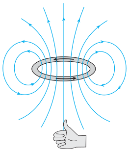
The figure depicts a single horizontal current loop — drawn as a flat ring or ellipse — carrying a steady current. Arrows on the loop indicate the direction of the current. Around the loop, blue magnetic field lines form closed loops that thread through the ring: they emerge upward from the top of the loop, fan outward, curve around the sides, and re-enter the bottom of the loop. This pattern is identical to the field of a bar magnet. The upper side of the loop is labelled as the north pole and the lower side as the south pole. Below the loop, a small stylised right hand is shown with fingers curled in the direction of the current and the thumb pointing upward — illustrating the right-hand thumb rule for the direction of the magnetic field.

Physical idea taught

The figure teaches that a current-carrying circular loop behaves like a magnetic dipole. The magnetic field lines are closed loops, just like those of a bar magnet. The direction of the field at any point is given by the right-hand thumb rule: if you curl the fingers of your right hand in the direction of the current, your thumb points in the direction of the magnetic field (out of the north pole). This analogy helps visualise the field pattern and understand that the loop has a north pole (where field lines emerge) and a south pole (where field lines re-enter).

Key formula developed with this figure

The textbook derives the magnetic field on the axis of a circular current loop using the Biot-Savart law. For a loop of radius $R$ carrying current $I$, the magnetic field at a point $P$ on the axis at distance $x$ from the centre is:

where:

• $\mu_0$ is the permeability of free space ($4\pi \times 10^{-7} \, \text{T m/A}$)
• $I$ is the steady current in the loop
• $R$ is the radius of the loop
• $x$ is the distance from the centre of the loop along the axis
• $\hat{\mathbf{i}}$ is the unit vector along the axis (direction given by the right-hand thumb rule)

At the centre of the loop ($x = 0$), the formula simplifies to: …