Mathematics · Ch 11 — Three-Dimensional Geometry

Distance Between Two Skew Lines

11.5.1

Distance Between Two Skew Lines

11.5.1 Distance Between Two Skew Lines

Understanding Skew Lines

Two lines in space that are neither parallel nor intersecting are called skew lines — they do not lie in the same plane and never meet. The shortest distance between them is the length of the segment perpendicular to both lines; this common perpendicular is unique.

Vector Form: Deriving the Shortest Distance Formula

Consider two skew lines:

l_1: \vec{r} = \vec{a}_1 + \lambda \vec{b}_1

l_2: \vec{r} = \vec{a}_2 + \mu \vec{b}_2

Here $\vec{a}_1$ is the position vector of a point $S$ on $l_1$ , $\vec{a}_2$ of a point $T$ on $l_2$ , and $\vec{b}_1$ , $\vec{b}_2$ are the direction vectors.

Let $\overrightarrow{PQ}$ be the shortest-distance segment. Being perpendicular to both lines, it is perpendicular to both $\vec{b}_1$ and $\vec{b}_2$ .

Important

The direction of the shortest distance vector is perpendicular to both $\vec{b}_1$ and $\vec{b}_2$ , so it is along $\vec{b}_1 \times \vec{b}_2$ .

The unit vector along the shortest distance is:

\hat{n} = \frac{\vec{b}_1 \times \vec{b}_2}{|\vec{b}_1 \times \vec{b}_2|}

Write $\overrightarrow{PQ} = d\,\hat{n}$ , where $d$ is the shortest distance. The vector $\overrightarrow{ST} = \vec{a}_2 - \vec{a}_1$ joins a point on $l_1$ to a point on $l_2$ , and $d$ equals the magnitude of the projection of $\overrightarrow{ST}$ onto $\hat{n}$ :

d = |\overrightarrow{ST} \cdot \hat{n}| = \left| (\vec{a}_2 - \vec{a}_1) \cdot \frac{\vec{b}_1 \times \vec{b}_2}{|\vec{b}_1 \times \vec{b}_2|} \right|

d = \frac{|(\vec{b}_1 \times \vec{b}_2) \cdot (\vec{a}_2 - \vec{a}_1)|}{|\vec{b}_1 \times \vec{b}_2|}

The numerator is the absolute value of the scalar triple product $[\vec{b}_1\;\vec{b}_2\;(\vec{a}_2 - \vec{a}_1)]$ .

Watch out

If $\vec{b}_1 \times \vec{b}_2 = \vec{0}$ , the lines are parallel (or coincident), not skew. This formula applies only when the cross product is non-zero.

Cartesian Form: Shortest Distance Between Skew Lines

Let the two skew lines be given in symmetric (cartesian) form:

l_1: \frac{x - x_1}{a_1} = \frac{y - y_1}{b_1} = \frac{z - z_1}{c_1}

l_2: \frac{x - x_2}{a_2} = \frac{y - y_2}{b_2} = \frac{z - z_2}{c_2}

with direction ratios $(a_1, b_1, c_1)$ and $(a_2, b_2, c_2)$ . Substituting $\vec{a}_1 = (x_1, y_1, z_1)$ , $\vec{b}_1 = (a_1, b_1, c_1)$ , $\vec{a}_2 = (x_2, y_2, z_2)$ , $\vec{b}_2 = (a_2, b_2, c_2)$ into the vector formula:

d = \frac{\left| \begin{vmatrix} x_2 - x_1 & y_2 - y_1 & z_2 - z_1 \\ a_1 & b_1 & c_1 \\ a_2 & b_2 & c_2 \end{vmatrix} \right|}{\sqrt{(b_1c_2 - b_2c_1)^2 + (c_1a_2 - c_2a_1)^2 + (a_1b_2 - a_2b_1)^2}}

The numerator is the determinant formed by the difference vector and the two direction vectors; the denominator is the magnitude of their cross product.

11.5.2 Distance Between Parallel Lines

Parallel lines are coplanar, so the distance between them is the perpendicular distance from any point on one line to the other. Let:

l_1: \vec{r} = \vec{a}_1 + \lambda \vec{b}

l_2: \vec{r} = \vec{a}_2 + \mu \vec{b}

sharing direction vector $\vec{b}$ , with $S$ on $l_1$ (position $\vec{a}_1$ ) and $T$ on $l_2$ (position $\vec{a}_2$ ).

Tip

For parallel lines, the shortest distance is the length of the perpendicular from any point on one line to the other. Choose the simplest point available.

Let $P$ be the foot of the perpendicular from $T$ onto $l_1$ , so the required distance is $|\overrightarrow{TP}|$ . With $\overrightarrow{ST} = \vec{a}_2 - \vec{a}_1$ and $\theta$ the angle between $\overrightarrow{ST}$ and $\vec{b}$ :

$|\overrightarrow{ST} \times \vec{b}| = |\overrightarrow{ST}|\,|\vec{b}|\,\sin\theta = |\overrightarrow{TP}|\,|\vec{b}|$ …

Figure 11.6Two skew lines l1 and l2 with points S and T, the join ST, and the common-perpendicular segment PQ giving the shortest distance, meeting both lines at right angles.

Fig. 11.6 — Two skew lines l1 and l2 with points S and T, the join ST, and the common-perpendicular segment PQ giving the shortest distance, meeting both lines at right angles.

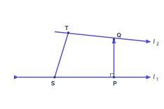
Drawn by us to help you understand the concept clearly, and verified to make sure it's accurate. For exams, practice from your textbook's own diagram.

Fig 11.6 is the key visual for understanding the shortest distance between two skew lines. It shows two non-parallel, non-intersecting lines in space — the defining property of skew lines. The lower line is labelled $l_1$ , the upper line $l_2$ , each drawn as an indigo arrow to indicate direction.

Two arbitrary points are marked: point $S$ on $l_1$ and point $T$ on $l_2$ , connected by a segment $ST$ . This segment is not perpendicular to either line — it is just any line joining a point on one skew line to a point on the other. The figure then introduces the critical feature: a segment $PQ$ that rises vertically from $P$ on $l_1$ to $Q$ on $l_2$ . This segment is drawn as an upward arrow, and it meets $l_1$ at a right angle. The text tells us $PQ$ is perpendicular to both $l_1$ and $l_2$ . That is the shortest distance segment — the unique line segment that is simultaneously orthogonal to both skew lines.

The physical idea is simple: among all possible segments joining a point on $l_1$ to a point on $l_2$ , the one that is perpendicular to both lines is the shortest. Any other segment, like $ST$ , is longer because it has a component along the direction of the lines. The figure makes this geometric fact concrete: $PQ$ is the "straightest" bridge between the two lines.

The textbook uses this figure to derive the formula for the shortest distance $d$ . The derivation proceeds as follows. Let the lines be given in vector form:

\vec{r} = \vec{a}_1 + \lambda \vec{b}_1 \quad \text{and} \quad \vec{r} = \vec{a}_2 + \mu \vec{b}_2

where $\vec{a}_1$ and $\vec{a}_2$ are position vectors of points on $l_1$ and $l_2$ (here $S$ and $T$ ), and $\vec{b}_1$ , $\vec{b}_2$ are direction vectors. The vector $\overrightarrow{PQ}$ is the shortest distance vector. Since it is perpendicular to both $\vec{b}_1$ and $\vec{b}_2$ , a unit vector along it is:

\hat{n} = \frac{\vec{b}_1 \times \vec{b}_2}{|\vec{b}_1 \times \vec{b}_2|}

Then $\overrightarrow{PQ} = d\,\hat{n}$ , where $d$ is the magnitude we want. Now consider $\overrightarrow{ST} = \vec{a}_2 - \vec{a}_1$ . The projection of $\overrightarrow{ST}$ onto $\hat{n}$ gives the component of $ST$ along the shortest distance direction. Since $PQ$ is exactly that component (the perpendicular drop), we have:

d = |\overrightarrow{ST} \cdot \hat{n}|

Substituting $\hat{n}$ gives the central formula:

d = \frac{|(\vec{b}_1 \times \vec{b}_2) \cdot (\vec{a}_2 - \vec{a}_1)|}{|\vec{b}_1 \times \vec{b}_2|}

In words: the shortest distance between two skew lines equals the absolute value of the scalar triple product of their direction vectors and the vector joining a point on each line, divided by the magnitude of the cross product of the direction vectors. The denominator $|\vec{b}_1 \times \vec{b}_2|$ is the area of the parallelogram formed by the two direction vectors; the numerator is the volume of the parallelepiped they span with $\vec{a}_2 - \vec{a}_1$ . The distance $d$ is the height of that parallelepiped — the perpendicular distance between the two lines. …

Start your 14-day free trial to unlock the full solution →

← Previous · 11.5Shortest Distance Between Two Lines Next · 11.5.2 →Distance Between Parallel Lines