Physics · Ch 8 — Mechanical Properties of Solids
Stress-strain Curve
Stress-strain Curve
The Stress-Strain Curve: What It Tells Us
When a solid is subjected to a deforming force, it undergoes a change in shape or size. The relationship between the stress (the internal restoring force per unit area) and the strain (the relative deformation) is not arbitrary — it follows a characteristic pattern that is captured by the stress-strain curve. This curve is obtained experimentally by gradually increasing the load on a specimen (say, a metal wire or a rod) and measuring the corresponding elongation or compression at each stage.
The curve is not a single straight line. It reveals several distinct regions, each corresponding to a different mechanical behaviour of the material. Understanding these regions is essential for predicting how a material will behave under load — whether it will spring back, deform permanently, or eventually break.
The Four Key Regions of the Curve
The stress-strain curve for a typical ductile material (like mild steel) can be divided into four main parts. We will go through them in the order they appear as stress increases.
1. Proportional Limit (Hooke's Law Region)
At very low stresses, the strain is directly proportional to the stress. This means the graph is a straight line passing through the origin. In this region, the material obeys Hooke's law:
The constant of proportionality is the Young's modulus (or the modulus of elasticity in general). So we write:
The point up to which this linear relationship holds is called the proportional limit. Beyond this point, the stress and strain are no longer proportional, and the graph begins to curve.
The proportional limit is not the same as the elastic limit (discussed next). It is simply the end of the linear region — the material may still be elastic for a little while longer.
2. Elastic Limit and Yield Point
After the proportional limit, the curve starts to deviate from a straight line. However, if the load is removed at any point before a certain critical stress, the material returns to its original dimensions. This critical stress is called the elastic limit.
- Elastic limit: The maximum stress that a material can withstand without permanent deformation.
- Yield point: For many materials (especially mild steel), there is a very clear stress at which the strain increases rapidly without any increase in stress. This is the yield point. The stress at this point is called the yield strength ().
At the yield point, the material "gives way" — it begins to flow plastically. The strain increases dramatically while the stress remains nearly constant. This flat region on the curve is called the yield plateau.
Do not confuse the elastic limit with the proportional limit. The elastic limit is always slightly higher than the proportional limit. The material is still elastic between these two points, but the stress-strain relation is no longer linear.
3. Plastic Region (Work Hardening)
Once the yield point is crossed, the material enters the plastic region. Here, the deformation is permanent — even if the load is removed, the material will not return to its original shape. The strain is now much larger than in the elastic region.
Interestingly, after the yield plateau, the curve begins to rise again. This happens because the material work-hardens (or strain-hardens). As the material is deformed plastically, its internal structure changes — dislocations in the crystal lattice multiply and tangle, making further deformation more difficult. So, to produce additional strain, a higher stress is required. The curve slopes upward, but less steeply than in the elastic region.
This region continues until the stress reaches a maximum value.
4. Ultimate Strength and Fracture
The highest point on the stress-strain curve is called the ultimate tensile strength (or simply ultimate strength, ). This is the maximum stress the material can withstand before it begins to fail.
After the ultimate strength is reached, a curious thing happens: the material starts to neck. A localised reduction in cross-sectional area occurs at some point along the specimen. Because the area decreases, the true stress in the necked region becomes very high, but the engineering stress (calculated using the original area) actually drops. The curve therefore turns downward.
Finally, at the breaking point (or fracture point), the material ruptures. The stress at which fracture occurs is called the breaking stress (). For ductile materials, the breaking stress is lower than the ultimate strength.
The ultimate tensile strength is the maximum stress on the engineering stress-strain curve. The breaking stress is the stress at actual fracture. For brittle materials, these two points are very close together — the material breaks soon after reaching its ultimate strength, with little or no plastic deformation.
Properties of the Stress-Strain Curve (as listed in the textbook)
The textbook lists several important properties that can be read directly from the curve. Each one is a quantitative measure of the material's mechanical behaviour.
›Proof
Property 1: Young's Modulus ()
In the linear (Hooke's law) region, the slope of the stress-strain curve gives the Young's modulus.
Let be the stress and be the strain. In the linear region:
Therefore,
This is a constant for a given material at a given temperature. A steeper slope means a stiffer material (higher modulus).
›Proof
Property 2: Yield Strength ()
The yield strength is the stress at the yield point. On the curve, it is the stress value at which the graph first shows a large increase in strain for a negligible increase in stress (the beginning of the yield plateau).
For materials that do not have a clear yield point (e.g., many aluminium alloys), the yield strength is often defined as the stress required to produce a specific amount of permanent strain, typically 0.2%. This is called the 0.2% offset yield strength.
›Proof
Property 3: Ultimate Tensile Strength ()
This is the maximum stress on the curve. It is the highest point of the graph. Mathematically, it is the maximum value of as a function of :
It represents the maximum load the material can support per unit original area.
›Proof
Property 4: Percentage Elongation (Ductility)
The total plastic strain at fracture, expressed as a percentage, is a measure of ductility. If the original length of the specimen is and the length at fracture is , then:
On the stress-strain curve, this corresponds to the total strain at the breaking point (minus the elastic strain, which is recovered upon unloading). A large percentage elongation indicates a ductile material; a small value indicates a brittle material.
›Proof
Property 5: Toughness
The toughness of a material is the total energy absorbed per unit volume before fracture. On the stress-strain curve, this is the area under the entire curve up to the breaking point.
If the curve is given by , then:
…
Drawn by us to help you understand the concept clearly, and verified to make sure it's accurate. For exams, practice from your NCERT textbook's own diagram.
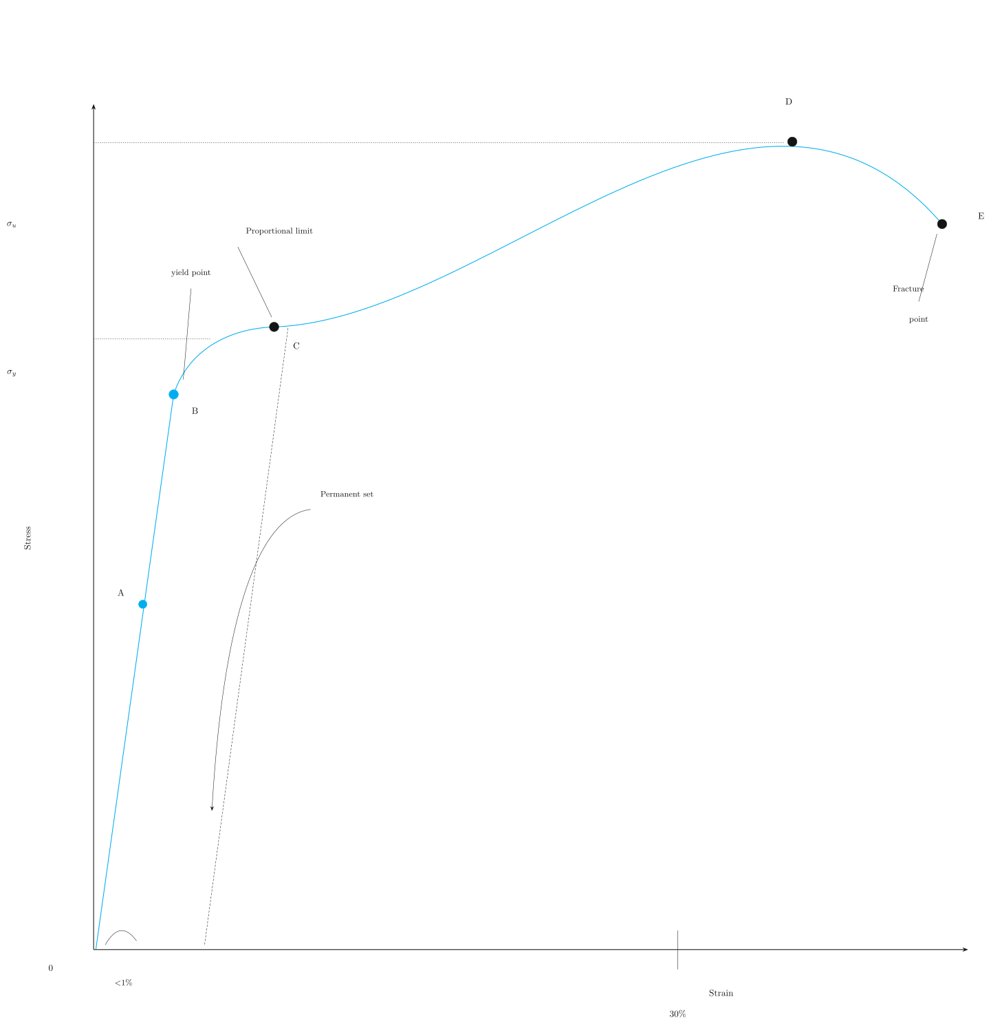
The figure plots stress (force per unit area, ) on the vertical axis against strain (fractional change in length, ) on the horizontal axis. The strain axis runs from 0 to about 30% — a huge range for a metal, which tells you this is a complete picture from loading all the way to breaking.
The curve starts at the origin O and climbs as a perfectly straight line up to point A. This straight segment is the proportional limit: up to A, stress and strain are directly proportional. That proportionality is Hooke’s law in action: , where is Young’s modulus. The slope of this straight line is Young’s modulus — the stiffness of the material.
Beyond A, the curve bends slightly. It reaches point B, labelled the yield point, with a corresponding stress marked on the y-axis. At B, the material begins to deform permanently: if you unloaded it here, it would not return to its original length. This is the elastic limit — the boundary between elastic and plastic behaviour.
The curve continues through point C, then rises to a peak at point D. The stress at D is the ultimate tensile strength, — the maximum stress the material can withstand. After D, the curve falls to point E, the fracture point, where the specimen breaks.
A dashed line drops vertically from point C down to the strain axis. That dashed line marks the permanent set: if you unload the material at C, it follows a straight line back to the strain axis (not back to the origin), and the strain remaining when stress reaches zero is the permanent deformation. The material has been stretched irreversibly.
Do not confuse the yield point B with the fracture point E. The yield point is where plastic flow begins; the fracture point is where the material separates. Between them lies the entire plastic region, including the peak at D. …
Drawn by us to help you understand the concept clearly, and verified to make sure it's accurate. For exams, practice from your NCERT textbook's own diagram.
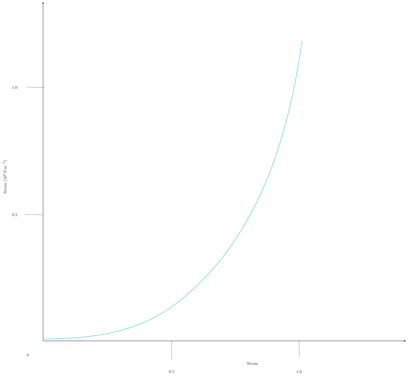
The aorta is not a metal rod or a steel beam — it is a soft, living tube that must stretch enormously to accommodate the surge of blood from each heartbeat. Figure 8.3 captures this behaviour directly.
The vertical axis is stress, measured in units of (megapascals, effectively), running from 0 to about 1.0. The horizontal axis is strain, a dimensionless ratio of extension to original length, also running from 0 to 1.0. A strain of 1.0 means the tissue has doubled in length — a huge deformation by engineering standards.
The curve itself is a single, smooth J-shape. Near the origin it is almost flat: a small stress produces a relatively large strain. This is the compliant, low-stiffness region where the elastic fibres in the aortic wall are being uncoiled and straightened. As strain increases, the curve begins to rise more steeply. By the time strain reaches about 1.0, the stress has climbed to roughly , and the slope is very steep indeed. There is no straight-line portion, no yield point, and no separate plastic region — the entire curve is one continuous nonlinear elastic response.
The key physical lesson is that biological tissues do not obey Hooke’s law. There is no single Young’s modulus for the aorta. Instead, the stiffness (the slope of the stress–strain curve) increases with strain. This is called strain-stiffening or a J-shaped stress–strain curve.
Why does this matter? At low strains the aorta is soft and expands easily, damping the pressure pulse from the heart. At high strains it becomes very stiff, preventing over-expansion and rupture. The textbook uses this figure to introduce the idea that the stress–strain relation is not a constant — it is a function of the strain itself.
The central formula that emerges from this discussion is not a single equation for the curve, but the definition of stress and strain that apply to any deformation, linear or not:
Here is the magnitude of the force applied perpendicular to the cross-section, is the original cross-sectional area, is the change in length, and is the original length. These definitions are universal — they hold whether the material is steel or aortic tissue. …